8 minutes
Do you know which inputs your neural network likes most?

Recent advances in training deep neural networks have led to a whole bunch of impressive machine learning models which are able to tackle a very diverse range of tasks. When you are developing such a model, one of the notable downsides is that it is considered a “black-box” approach in the sense that your model learns from data you feed it, but you don’t really know what is going on inside the model.
To make it clearer: you don’t really know what your model actually learned and if you have a flaw in your training / data approach it might work well according to your metrics while having learnt the wrong thing. As a self-respecting developer you want to do better than that, so today I will show you a method you can use to get some better introspection into your model by using visualization techniques.
So what is a visualization techniqe when we talk about deep neural networks?
The basic idea of visualization is that you try to figure out what your network is tuned towards by letting it manipulate your input image to make the image as “exciting” as possible for the network. It’s kind of like letting a kid decide which and how much ice cream it wants to have - you will end up with 9 scoops of all flavors.
Let’s look at the ice cream flavors and scoops of an example neural network. To make it easy, I’ll focus on the well-known MNIST problem in PyTorch to make sure it is easy for everyone to have an intuition and figure out what the visualization can show us.
Example PyTorch network: MNIST classification
So, first, we will need to code to train a PyTorch network for MNIST - of course as this is a simple problem we don’t need a very deep network, but the techniques presented here can be used for very deep ones in the same way, so I consider this a positive thing.
In MNIST, the task of the network is to classify the written digits 0 - 9 in images.
Example images look like this:
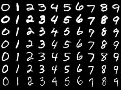
Example MNIST hand-written digits
I used the PyTorch code for MNIST from the examples repository which consists of two convolutional layers followed by two fully connected layers. When training it for 10 epochs on 60000 examples, it achieved 99% accuracy, so it is working well enough.
Visualization Intuition
When we are training a neural net we are using the method of backpropagation to change the weights of our network with respect to the error gradients we receive going backwards from our output. The input image is fixed in this respect and the weights of the network are variable.
In visualization we are doing the exact opposite: we are keeping the weights of our network fixed to evaluate a given model and then use backpropagation to change the input image to get “better” results of our network. And this “better” results is where several possibilities kick in. We could be interested in finding out which input image our network considers most appropriate when we want to find out a specific class, e.g. the digit 5 in our MNIST example. The task then becomes: create an image which leads the network to output the class 5 as much as possible.
Visualization Implementation
After loading our trained model weights, we need to make sure that our network is fixed, so its weights don’t change when we use backpropagation. To do so we call model.eval() which makes sure that the weights of the model will not be changed when backpropagating:
model = Net()
model.load_state_dict(torch.load('./mnist_cnn.pt'))
model.eval()  # Don't change model weights
On the other hand, we want the algorithm to change the input image to excite the network more and more, so we need to make sure that the input image can be adjusted. To do so we make sure that the input image is a PyTorch tensor with requires_grad equal to True.
This is PyTorch’s way of saying that a tensor should have tunable values which are influenced when running backpropagation. If you want to know more about how PyTorch does that, check out the well-written documentation.
As we are dealing with MNIST here, we start with an input image consisting of zeros which is the representation for all black pixels, so we start with a totally black image with only 1 color channel and 28 by 28 pixels:
img = np.uint8(np.zeros((1, 28, 28)))
We then run 50 iterations where we change the input image a little bit in each iteration to better match what the neural net finds exciting given the class (for example the number 5) we are currently interested in. So how do we do that?
Our model uses log_softmax for the output which means that first a softmax function is applied which makes sure that the sum of all the outputs is equal to 1 and then the logarithm is applied. The better our network classifies, the more the correct target number will be equal to 1 in the softmax and the non-targets will be small numbers. The logarithm of 1 is equal to 0, so the better our network is, the more the output for the target number will be 0. In contrast, the non-targets are small positive numbers after the softmax which will be turned into larger negative numbers by the logarithm.
We can use these properties to construct a loss which is lower both when the network is very sure about the target number, but also when it is very sure that the non-targets are unlikely.
If this is the case, the target number will be 0 and the others larger negative numbers.
So for the loss we can use: loss = -10 * output[0, target_class] + torch.sum(output) which multiplies the target number with -10 to punish it, if it is not 0 and sums the other numbers which are negative. The more negative they get, the lower the loss, which is what we want.
So let’s use that constructed loss:
for i in range(num_loops):
    tensor = img_to_tensor(img)
    optimizer = Adam([tensor], lr=lr)
    output = model(tensor)
    loss = -10 * output[0, target_class] + torch.sum(output)
    model.zero_grad()
    loss.backward()
    optimizer.step()
    img = tensor_to_img(tensor)
In each iteration, we convert our current image (starting with a completely black image) to a PyTorch tensor and letting our optimizer know that we want to change this tensor. We pass it into the model to obtain the output and then construct the loss as just discussed. We then backpropate from that loss to calculate the gradients and then adjust our parameters (i.e. the input image) by taking a step() in the optimizer. Finally, we convert the tensor back to an image, so we can save it to take a look.
The function img_to_tensor just transforms the pixel values that are integers in the range 0-255 to a PyTorch tensor in batch format by dividing by 255 and then subtracting the MNIST mean and dividing by the standard deviation. In addition it makes sure that requires_grad is set to True, so we can change this tensor:
def img_to_tensor(img):
    img_float = np.float32(img)
    img_float[0] /= 255
    img_float[0] -= MNIST_MEAN
    img_float[0] /= MNIST_STD
    img_tensor = torch.from_numpy(img_float).float()
    img_tensor.unsqueeze_(0)  # Make a batch
    img_tensor.requires_grad_()
    return img_tensor
The function tensor_to_img in contrast does the inverse: it multiplies by the standard deviation and adds the mean and then multiplies by 255 to get an integer image back which we can then visualize:
def tensor_to_img(img_variable):
    img = copy.copy(img_variable.data.numpy()[0])
    # Inverted restoration of std / mean
    img[0] *= MNIST_STD
    img[0] += MNIST_MEAN
    img[img > 1] = 1
    img[img < 0] = 0
    img = np.round(img * 255)
    return img
You can find all of this code in my PyTorch visualization Github repository.
This is really all that we need, so let’s check out what we get from this.
Results of the visualization for MNIST
Here are the resulting images the network is most tuned towards for the 10 target classes (numbers 0-9) after 50 iterations:
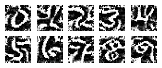
Images the network is most tuned towards for the 10 different target numbers
As you can see, you can make out the numbers rather clearly, so the network seems to have learned the right thing. For me, number 1 looks a bit weird, so it might be that there is the highest variance when drawing a 1 in comparison to other numbers. It could also be that you can improve the network further by analyzing this effect further.
Visualizing the deeper parts
So far, we asked the high-level question: how does an input image look like to excite the network most. Another interesting question we can ask is: What do the inputs for the different channels in our layers look like that excite these channels most?
To do this, we need to use so-called hooks to find out the inputs and outputs to these inner parts and then tune the network several times to maximally excite this, but I’ll save this for another blog post.
Further possibilities
Of course, this blog post only scratches the surface of what you can do. You need to go deeper.

We need to go deeper
You can visualize the actual inputs each part of the network receives when you present it with a particular image, you can use more advanced techniques to better visualize the network etc.
If you want to know more, leave a comment, so I consider to write another post about this topic.
python pytorch machinelearning deeplearning visualization
Machine Learning Deep Learning Visualization
1574 Words
December 30, 2019