9 minutes
Meta-learning from noisy labels
Label noise introduction
Training machine learning models requires a lot of data. Often, it is quite costly to obtain sufficient data for your problem. Sometimes, you might even need domain experts which don’t have much time and are expensive.
One option that you can look into is getting cheaper, lower quality data, i.e. have less experienced people annotate data. This usually has the side effect of your labels becoming more noisy.
Then you can collect a high-quality subset of your data using trained professionals, so you are confident that the labels are as correct as humanly possible.
This blog post dives into a meta-learning method which uses a high-quality subset of your data to guide the training of the larger noisy training dataset by assigning weights to each data point. It’s based on the paper “Learning to reweight examples for robust deep learning” by Ren et al.
Meta-learning can be considered as “learning to learn”, so you are optimizing some parameters of the normal training step. In a sense this means that you have a two-step backpropagation which of course is more computationally expensive.
Learning to reweight examples for robust deep learning
So let’s check out the idea from the paper. Let’s name our noisy training dataset as X_noisy and our clean high-quality dataset as X_clean.
Of course, the number of examples in X_noisy is much much larger than the number of examples in X_clean.
The idea is that X_clean will be used to find out which data points from X_noisy are likely noisy and assign low weights to them during training, so we discard them and only train with the ones that have the correct labels.
How can this be done?
It’s quite easy to understand: during training, you calculate the loss for each example in your training batch and assign a zero weight to each of them. Assigning a zero weight means your loss would be zero, so you would not update the model and not learn anything. The trick is then to take a batch from your clean dataset and calculate the loss on it (all data points equally weighted with ones). Then you try to reduce the loss of the clean dataset with respect to the weights of your training batch, i.e. you try to shift the weights, so that the resulting training step would shift the model in the direction as to reduce the loss of your clean set. This can be done by calculating the derivative of the clean set loss with respect to the weights of the noisy dataset.
So essentially, the clean dataset figures out how it would benefit from learning from each of the noisy samples. If taking a noisy sample into account would lead to the loss of the clean dataset increasing, then we don’t want to do that, so we would keep the weight at 0. If, however, taking a noisy sample into account would lead to a decrease of the loss of the clean dataset, that’s exactly what we want, so we would increase the weight of that datapoint.
The meta-learning part about this is that we need to ask the question: how would the optimization of the model change if we assign different weights, so we need to figure out the optimal weight assignment that drives the model learning (the normal backpropagation) in the direction of helping our clean dataset.
Code implementation and comparison with regular training
Let’s codify this to make it fully clear and understandable. There is a great open-source library called higher that helps us to implement such a meta-learning approach while keeping our code super clean.
For this experiment, we will be using the MNIST dataset which is an image classification dataset with 10 different classes. It contains images of size 28x28 pixels and has 6000 per class for training and 1000 per class for the test set.
It’s an easy problem which can be solved with simple networks and is fast to train, so it’s a good candidate to introduce severe noise for our setup.
Data loading and noise generation
Let’s setup our data loading:
import torchvision
import torch
import torch.nn as nn
import torch.nn.functional as F
import torchvision.transforms as transforms

stats = ((0.1307,), (0.3081,))
transforms = transforms.Compose(
    [transforms.ToTensor(),
     transforms.Normalize(*stats)])
train_data = torchvision.datasets.MNIST(
    root='/home/marc/.pytorch-data', download=True, train=True, transform=transforms)

test_data = torchvision.datasets.MNIST(
    root='/home/marc/.pytorch-data', download=True, train=False, transform=transforms)
We’ll use a super simple fully connected network which is normally sufficient to get high accuracy results on MNIST:
model = nn.Sequential(nn.Linear(784, 128),
                      nn.ReLU(),
                      nn.Linear(128,64),
                      nn.ReLU(),
                      nn.Linear(64,10)).cuda()
MNIST itself is not a very noisy dataset, so first, let’s add a lot of noise and get our noisy and clean set. We’ll create 80% noise, so 80% of our labels will be changed to some random other class. For the clean set, we’ll keep 50 examples per class, so a tiny portion of our data.
import copy
import random
import numpy as np

def create_noisy_dataset(original, extract_clean_per_class=50, noise_ratio=0.8):
        num_classes = len(original.classes)
        targets = np.array(original.targets)
        clean_targets = clean_data = noisy_targets = noisy_data = None
        for cls in range(num_classes):
            class_mask = targets == cls
            new_clean_targets = targets[class_mask][:extract_clean_per_class]
            new_noisy_targets = targets[class_mask][extract_clean_per_class:]
            num_noisy = int(noise_ratio * new_noisy_targets.shape[0])
            random_noise = np.random.randint(0, num_classes, num_noisy)
            other_classes = [i for i in range(num_classes) if i is not cls]
            random_noise[random_noise == cls] = random.choice(other_classes)
            new_noisy_targets[:num_noisy] = random_noise
            new_clean_data = original.data[class_mask][:extract_clean_per_class]
            new_noisy_data = original.data[class_mask][extract_clean_per_class:]
            if clean_targets is None:
                clean_targets = new_clean_targets
                clean_data = new_clean_data
                noisy_targets = new_noisy_targets
                noisy_data = new_noisy_data
            else:
                clean_targets = np.concatenate([clean_targets, new_clean_targets])
                clean_data = torch.cat([clean_data, new_clean_data])
                noisy_targets = np.concatenate([noisy_targets, new_noisy_targets])
                noisy_data = torch.cat([noisy_data, new_noisy_data])
        clean = copy.deepcopy(original)
        clean.data = clean_data
        clean.targets = clean_targets
        noisy = copy.deepcopy(original)
        noisy.data = noisy_data
        noisy.targets = noisy_targets
        combined = copy.deepcopy(original)
        combined.data = torch.cat([clean_data, noisy_data])
        combined.targets = np.concatenate([clean_targets, noisy_targets])
        return clean, noisy, combined
Using this noise creation helper, we’ll setup the data and our dataloaders:
import itertools
from torch.utils.data import DataLoader

clean_data, noisy_data, combined_data = create_noisy_dataset(train_data)

combined_train_loader = DataLoader(combined_data, batch_size=128, shuffle=True, num_workers=6)
clean_loader = DataLoader(clean_data, batch_size=128, shuffle=True, num_workers=6)
clean_loader_loop = itertools.cycle(clean_loader)
train_loader = DataLoader(noisy_data, batch_size=128, shuffle=True, num_workers=6)
test_loader = DataLoader(test_data, batch_size=128, shuffle=False, num_workers=6)
To verify if this worked correctly, we’ll plot a few examples:
import matplotlib.pyplot as plt

for images, targets in combined_train_loader:
    for i in range(18):
        plt.subplot(3,6,i+1)
        plt.imshow(images[i][0], cmap='gray')
    plt.show()
    print(targets[:6])
    print(targets[6:12])
    print(targets[12:18])
    break
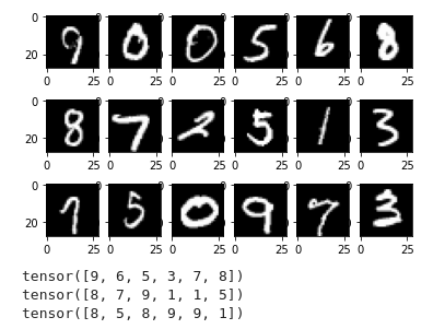
Examples of our generated noisy data
Baseline - regular training
As a baseline, let’s train our network without meta-learning. To try to make it a fair comparison we combine the noisy set and the clean set and use both of them for training in our combined_data_loader:
import time

model = nn.Sequential(nn.Linear(784, 128),
                      nn.ReLU(),
                      nn.Linear(128,64),
                      nn.ReLU(),
                      nn.Linear(64,10)).cuda()
optimizer = torch.optim.Adam(model.parameters(), lr=0.0006)

for epoch in range(25):
    start_epoch = time.time()
    correct = 0
    for images, labels in combined_train_loader:
        optimizer.zero_grad()
        predictions = model(images.cuda().reshape(-1, 28*28))
        loss = F.cross_entropy(predictions, labels.cuda())
        loss.backward()
        optimizer.step()
        correct += (torch.argmax(predictions, dim=1) == labels.cuda()).sum().item()
    print(f"Epoch {epoch} took {time.time() - start_epoch: {3}.{4}}s")
    print(f"Train loss: {loss.item(): {3}.{4}}")
    print(f"Train accuracy: {100 * correct / len(train_data): {3}.{4}}%")
    with torch.no_grad():
        model.eval()
        correct = 0
        for images, labels in test_loader:
            predictions = model(images.cuda().reshape(-1, 28*28))
            correct += (torch.argmax(predictions, dim=1) == labels.cuda()).sum().item()
        print(f"Test accuracy: {100 * correct / len(test_data): {3}.{4}}%")
Epoch 0 took  1.791s
Train loss:  2.254
Train accuracy:  17.39%
Test accuracy:  68.96%
Epoch 1 took  1.821s
Train loss:  2.197
Train accuracy:  19.21%
Test accuracy:  73.77%
Epoch 2 took  1.839s
Train loss:  2.263
Train accuracy:  20.02%
Test accuracy:  72.16%
...
Epoch 22 took  1.823s
Train loss:  1.993
Train accuracy:  29.02%
Test accuracy:  44.01%
Epoch 23 took  1.83s
Train loss:  2.074
Train accuracy:  29.66%
Test accuracy:  42.44%
Epoch 24 took  1.837s
Train loss:  1.98
Train accuracy:  29.83%
Test accuracy:  40.44%
When we visualize these accuracies, it looks like this:
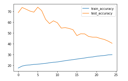
Plotting the accuracies of the regular training over epochs
As you can see, our network continues to improve on the training data while suffering on the test data, so it is overfitting. After 25 epochs, we only get a test set accuracy of around 40%. And if we had stopped early at our best epoch, the test set accuracy was 74%.
Meta-learning implementation
For our meta-learning training with the clean set as guidance, we need to make the following changes:
- We are using a
withblock with thehigherlibrary to be able to run a meta step. - We keep the individual loss items by using
reduction='none'. - We add zero weights for every noisy item (
eps) that we then tune using our clean set. - We run a normal step on our clean set and then calculate the gradients of the resulting loss with regards to the weights
eps. - We normalize the weights after making sure that the minimum weight is 0.
- This completes the meta step, so afterwards we simply run our normal training step, but use the weights we determined in the meta step.
And in code it looks like this:
import higher

model = nn.Sequential(nn.Linear(784, 128),
                      nn.ReLU(),
                      nn.Linear(128, 64),
                      nn.ReLU(),
                      nn.Linear(64, 10)).cuda()
optimizer = torch.optim.Adam(model.parameters(), lr=0.0006)

for epoch in range(25):
    start_epoch = time.time()
    model.train()
    correct = 0
    for images, labels in train_loader:
        optimizer.zero_grad()
        with higher.innerloop_ctx(model, optimizer) as (fmodel, diffopt):
            predictions = fmodel(images.cuda().reshape(-1, 28*28))
            loss = F.cross_entropy(predictions, labels.cuda(), reduction='none')
            eps = torch.zeros_like(loss, requires_grad=True)
            eps_weighted_loss = torch.sum(loss * eps)
            diffopt.step(eps_weighted_loss)

            clean_images, clean_labels = next(clean_loader_loop)
            predictions_clean = fmodel(clean_images.cuda().reshape(-1, 28*28))
            loss_clean = F.cross_entropy(predictions_clean, clean_labels.cuda())
            grad_eps = torch.autograd.grad(loss_clean, eps)[0].detach()

        weights = torch.clamp(-grad_eps, min=0)
        weight_sum = torch.sum(weights)
        if weight_sum > 0:  # avoid zero division
            weights = weights / weight_sum

        predictions = model(images.cuda().reshape(-1, 28*28))
        loss = F.cross_entropy(predictions, labels.cuda(), reduction='none')
        loss = torch.sum(weights * loss)
        loss.backward()
        optimizer.step()

        correct += (torch.argmax(predictions, dim=1) == labels.cuda()).sum().item()
    print(f"Epoch {epoch} took {time.time() - start_epoch: {3}.{4}}s")
    print(f"Train loss: {loss.item(): {3}.{4}}")
    print(f"Train accuracy: {100 * correct / len(noisy_data): {3}.{4}}%")
    with torch.no_grad():
        model.eval()
        correct = 0
        for images, labels in test_loader:
            predictions = model(images.cuda().reshape(-1, 28*28))
            correct += (torch.argmax(predictions, dim=1) == labels.cuda()).sum().item()
        print(f"Test accuracy: {100 * correct / len(test_data): {3}.{4}}%")
Epoch 0 took  4.656s
Train loss:  1.647
Train accuracy:  17.63%
Test accuracy:  83.83%
Epoch 1 took  4.533s
Train loss:  0.9988
Train accuracy:  18.71%
Test accuracy:  84.66%
Epoch 2 took  4.733s
Train loss:  1.619
Train accuracy:  18.88%
Test accuracy:  85.1%
...
Epoch 22 took  4.727s
Train loss:  2.008
Train accuracy:  20.63%
Test accuracy:  85.25%
Epoch 23 took  4.787s
Train loss:  1.65
Train accuracy:  20.77%
Test accuracy:  85.30%
Epoch 24 took  4.735s
Train loss:  1.358
Train accuracy:  20.83%
Test accuracy:  85.36%
Visualizing the accuracies here, gives us:
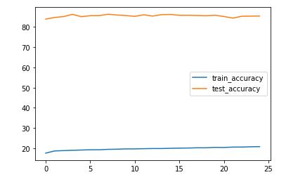
Plotting the accuracies of the meta-learning approach over epochs
Conclusion
As you can see, it now looks as it should - the training accuracy stays low around 20% as it’s mostly noisy data, so when we predict correct targets, they should be mostly wrong. In contrast, we are making good progress on the test set and reach an accuracy of around 85% after 25 epochs. In particular, the training is now not overfitting and our results are better than during the normal training even when using early stopping.
Our clean set really guided the training in the right direction :)
One final note, though: this definitely comes at a cost. If you look at the epoch duration, the meta-learning approach is about 2,5-3 times slower than the normal training.
References
Mengye Ren, Wenyuan Zeng, Bin Yang, Raquel Urtasun: Learning to Reweight Examples for Robust Deep Learning
python machinelearning deeplearning pytorch paper labelnoise
Machine Learning Deep Learning Deep Learning Papers
1847 Words
June 25, 2021