Training a simple neural network in Numpy

In this post, I am going to show you how easy it is to train a basic neural network in plain Python with Numpy, i.e. without using fancy libraries like Tensorflow or PyTorch. I think it is important to grasp what is going on without using a framework to understand how the frameworks help you out and what exactly they handle for you. Also, it is nice to see that you have a full understanding of what you are dealing with, so let’s get started.

Build the ReLU activation function

We’ll start by building the often used ReLU (rectified linear unit) activation function which our neurons are using as their non-linear activation part. Without a non-linear function, we would only be able to model linear relations which is much less powerful.

import matplotlib.pyplot as plt
import numpy as np
%matplotlib inline

def relu(x):
    return np.maximum(x, 0)
    
x = np.linspace(-5, 10)
plt.plot(x, relu(x))

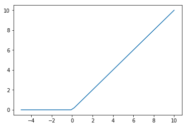
As you can see, ReLU - while sounding fancy - is really just one line of code np.maximum(x, 0).

Define the basic parameters

We will use a batch_size of 128 data points with each data point consisting of 1000, dimensions, i.e. 1000, numbers which should be transformed to 1 final number. You can think of this as 1000, pixels of an image which we want to map to a single category (cat / dog). Our network will use 100, so-called hidden neurons because they are not visible in our data.

batch_size = 128
input_dim = 1000
hidden_dim = 100
output_dim = 1

Create random input and target values

For this example, we are not using real data, but just fake some random data, so let’s generate inputs and random outputs:

input_values = np.random.randn(batch_size, input_dim)
output_values = np.random.randn(batch_size, output_dim)

Create random weights for the network

Our network needs to have weights which are the trainable parameters of it. We initialize them at random as well mapping from the input to the hidden neurons and from the hidden to the output neurons.

weights1 = np.random.randn(input_dim, hidden_dim)
weights2 = np.random.randn(hidden_dim, output_dim)

Check out the random performance before training

Now, how does our network perform at random? To evaluate, we multiply our input values with the first layer weights of the network and apply the ReLU activation function. That result is the input to the next layer, so it is multiplied by the second layer weights. We subtract the resulting output from our expected outputs (which were randomly generated as well).

layer1_activations = input_values.dot(weights1)
layer1_relu = relu(layer1_activations)
predictions = layer1_relu.dot(weights2)

print(predictions[:5] - output_values[:5])

[[ 19.41335228]
[-114.82687673]
[ -48.65366846]
[ -83.93903766]
[ -45.05468704]]

As we can see here, the difference between the neural network activation and the target output values is high, so the network is not really helpful. This makes sense as we haven’t trained it, yet!

Train the network

We train the network for 1000, iterations by calculating its output as described above yielding the predictions. Then, our loss is the sum of all the squared differences between the predictions and our target values. The gradients are derived from basic calculus, but the good news is if this is too much Math for you: this is exactly what frameworks such as Tensorflow or PyTorch do for us. They automatically calculate the gradients for the backward propagation, so you do not need to do the Math. Finally, we use the gradients combined with our small learning rate to shift our weights in the right direction using gradient descent.

num_loops = 1000
learning_rate = 1e-6
for i in range(num_loops):
    activations = input_values.dot(weights1)
    relu_activations = relu(activations)
    predictions = relu_activations.dot(weights2)
    
    loss = np.sum((predictions - output_values) ** 2)
    if ((i <= 100) & (i % 10, == 0) | (i % 100, == 0)):
        print(i, loss)
    
    # Gradients
    dloss_predictions = 2.0, * (predictions - output_values) 
    dloss_weights2 = relu_activations.T.dot(dloss_predictions)
    dloss_relu_activations = dloss_predictions.dot(weights2.T)
    dloss_activations = dloss_relu_activations.copy()
    dloss_activations[activations < 0] = 0
    dloss_weights1 = input_values.T.dot(dloss_activations)
    
    # Gradient Descent
    weights1 -= learning_rate * dloss_weights1
    weights2 -= learning_rate * dloss_weights2

(0, 3107119.8819272295)
(10, 6477731.174215912)
(20, 503218.95979508833)
(30, 186387.32762751653)
(40, 87792.08797737992)
(50, 45913.89335566323)
(60, 25153.979455418485)
(70, 14326.035509846992)
(80, 8452.117490799272)
(90, 5143.63172174059)
(100, 3218.3550710330437)
(200, 141.09191752470858)
(300, 59.34055206962512)
(400, 58.5022453137973)
(500, 58.49755563734828)
(600, 58.49744545275112)
(700, 58.49744260872595)
(800, 58.49744253070574)
(900, 58.49744252846752)\

As you can see, the loss gets smaller and smaller during the training iterations.

Checkout the performance after training

layer1_activations = input_values.dot(weights1)
layer1_relu = relu(layer1_activations)
predictions = layer1_relu.dot(weights2)

print(predictions[:5] - output_values[:5])

[[ 8.12997038e-05]
[ -2.77850692e-01]
[ 1.24521122e-04]
[ 5.35664771e-05]
[ -3.48770488e-04]]

The difference is now very close to 0 (8.1e-05 = 0.000001), so our network successfully learned good weights to map our input values to our output values. We probably overfitted the network, i.e. it is now very tuned to the specific data we fed it, but that is the topic for another blog post.

This is how easy it is to write a neural network in Python with Numpy. For a more advanced article about neural networks check out how to play video using deep Q learning.