8 minutes
Accurate, Large Minibatch SGD: Training ImageNet in 1 Hour

New blog series: Deep Learning Papers visualized
This is the first post of a new series I am starting where I explain the content of a paper in a visual picture-based way. To me, this helps tremendously to better grasp the ideas and remember them and I hope this will be the same for many of you as well.
Today’s paper: Accurate, Large Minibatch SGD: Training ImageNet in 1 Hour by Goyal et al.
The first paper I’ve chosen is well-known when it comes to training deep learning models on multiple GPUs. Here is the link to the paper of Goyal et al. on arxiv. The basic idea of the paper is this: when you are doing deep learning research today, you are using more and more data and more complex models. As the complexity and size rises, of course also the computational needs rise tremendously. This means that you typically need much longer to train a model to convergence. But if you need longer to train a model, your feedback loop is long which is frustrating as you already get many other ideas in the mean time, but as it takes so long to train, you cannot try them all out. So what can you do?
You can train on multiple GPUs at the same time and in theory get results faster the more GPUs you use. Assume you need 1 week to train your model on a single GPU, then with 2 GPUs in parallel, you should be able to achieve the same training in about 3.5 days and when using 7 GPUs you only need a day.
So how does it work to train your model on multiple GPUs? Typically, data parallelization is used which simply means that when you have your epoch, you send some distinct data to each distinct GPU. But then how do you get a model that benefits from all the data? Basically, you always synchronize the gradients, so after each batch, you collect the gradients from each GPU, calculate the average of the gradients over all GPUs and then adjust the model weights.
Let’s take a visual look at this:
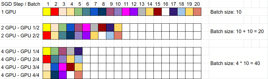
Training the same amount of data on 1 vs 2 vs 4 GPUs
Increasing the batch size -> increasing the learning rate
Note what happens when you do this: your batch size is rising! Let’s say you have 200 images per epoch and your batch size is 10. Then for a single GPU, you have 20 batches per epoch à 10 images. If you train on 2 GPUs, then your batch size is twice the size: 20. That’s because each of your two GPUs gets 10 images and calculates the gradients of those 10 and then you take the average of the gradients of those 2 GPUs, so your gradients are averaged over 20 images. This means that your epoch now only has 10 batches per epoch à 20 images. So by increasing the batch size, your are also reducing the number of batches per epoch and this in turn is exactly why it’s almost (except for the synchronization overhead) twice as fast to train. Similarly, if you were to use 4 GPUs, then each GPU receives 10 images per batch, so your effective batch size is 40. Thus, you only need 5 batches per epoch to train your 200 images.
But in turn, if you only use 5 batches per epoch instead of 20, that also means that you are only taking 5 gradient descent steps instead of 20 on a single GPU. We need to take a look what that means:
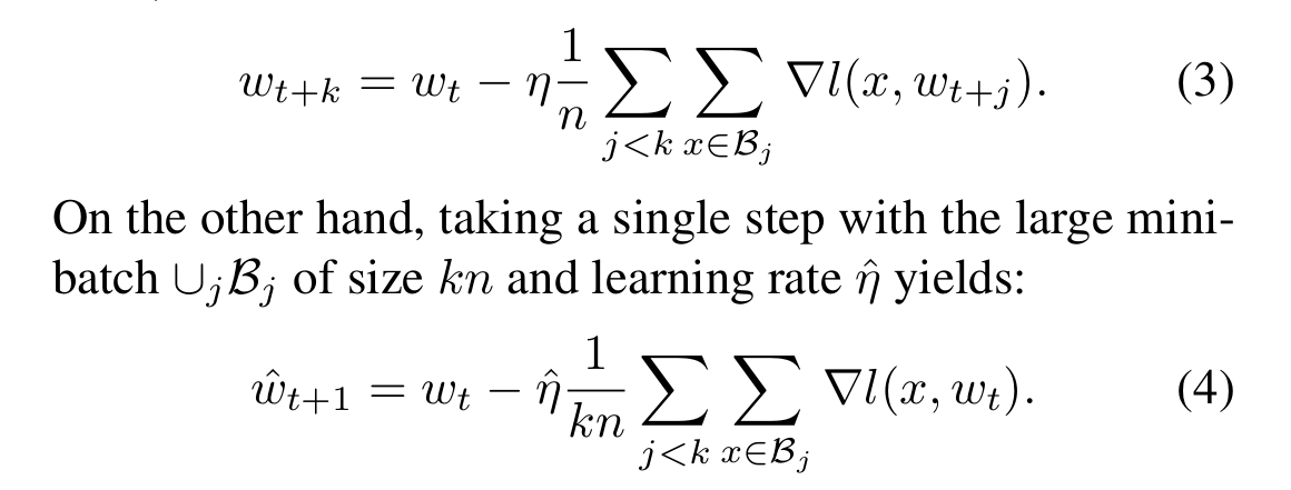
Equations 3 and 4 from the paper
Equation 3 represents the single GPU case after k iterations, in our case let’s take k = 4, so after 4 batches. This means we were updating our weights 4 times which is the first sum with j < k, so j=0, j=1, j=2 and j=3. The second sum is the loop over the images in the corresponding batch and we calculate the gradient ($\nabla l$) determined by our weights at that time t+j and the image example x. We divide everything by n which is just the batch size, so n=10 in our example case and multiply by the learning rate $\eta$.
In contrast, equation 4 represents the multi GPU case for 4 GPUs (as we had k = 4). The 4 GPUs only take a single gradient descent step as the batch size is 4 times as large ($kn=4*10=40$). In this case, the first sum with j < k is over our 4 GPUs and the seconds sum over the batch of each individual GPU. As we take the average of all of these, we divide by $kn=40$. This means that our step is k times smaller.
Now, the main idea of the paper is that we can make sure that the step size is roughly the same by scaling up our learning rate by the number of GPUs we are using: $\hat{\eta}=k * \eta$. By doing so, equations 3 and 4 become roughly the same, because $\hat{\eta} * \frac{1}{kn} = k*\eta * \frac{1}{kn} = \eta * \frac{k}{kn} = \eta * \frac{1}{n}$.
Or to visualize:
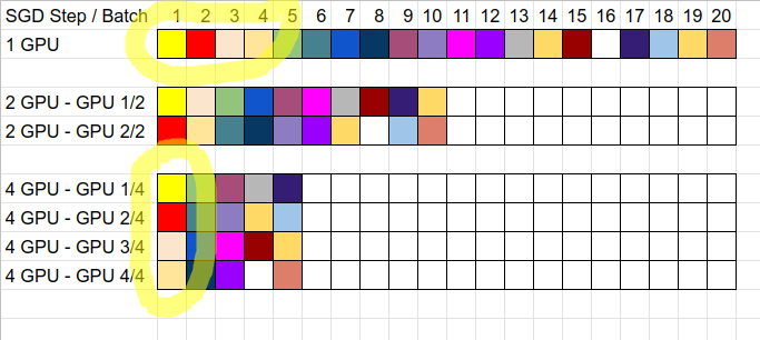
Four SGD steps on a single GPU is a single step with four GPUs
Intuition
To summarize so far: when we increase the number of GPUs to train with, we are increasing the effective batch size which leads to less batches per epoch and thus less SGD training steps. To compensate for less steps, we need to scale the learning rate linearly. This is simple: multiply the original single GPU learning rate by the number of GPUs you are using to train now. For example if your learning rate was 1e-3 before with a single GPU and now you train with 4 GPUs, then simply increase it to 4e-3.
Why does it intuitively make sense to scale the learning rate?
When your batch size is larger you will get a better estimate of the direction of the gradient in the right direction -> your gradients are less fuzzy. Thus, when you have a more representative gradient, it makes sense to be able to take a larger step as the likelihood of walking in the wrong direction is reduced by the larger sample of examples.
Here is an illustration with the single GPU model taking 4 small steps (yellow) and the 4 GPU model taking 1 larger step (blue; the learning rate is multiplied by 4, so the step is four times as large):
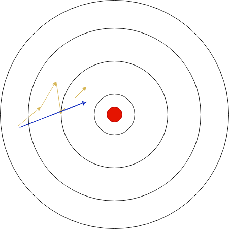
Illustration of gradient steps in the weight space. Red circle is the target / optimal weight configuration. Starting from a weight initialization in the left of the image, the single GPU model (yellow) takes 4 noisy steps. In contrast, the 4 GPU model (blue) takes a single larger step in a better approximated direction.
Problem: initial large learning rates
The authors note that the learning process is most vulnerable in the beginning, because the weights are initialized at random and steps in the wrong direction can lead to a suboptimal space. Thus, they argue that the learning rate should not be immediately set to the higher value, but rather a learning rate annealing schedule should be used, so it starts low and then increases over time.
They try out different warm-up schedules and conclude that it works best to warm-up over 5 epochs, so that after 5 epochs the maximal learning rate is reached. However, I already observed machine learning models where a longer warm-up period is required, so you should try it out for your own problem.
How does this look like in practice? Assume your learning rate for single GPU training is 1e-3. So you want to end up at 4e-3 when training with 4 GPUs. So you need to add the learning rate (4-1) times to itself over 5 epochs: $lr_{epoch} = lr_{single-gpu} + lr_{single-gpu} * (n-1) * (epoch / 5)$. Here, $lr_{epoch}$ is the learning rate to use in a given epoch, $lr_{single-gpu}$ is the initial learning rate, n is the number of GPUs and epoch is your epoch.
And this is how this warm-up looks like over epochs:
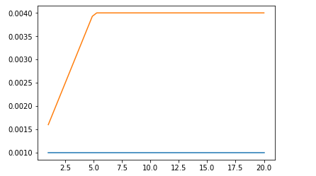
Learning rate gradual warmup (orange) for 4 GPUs vs. constant learning rate for a single GPU (blue).
Summary
While the paper goes into more details, I discussed the most practical aspects of it and tried to visualize the key parts.
In particular, when training your machine learning model with multiple GPUs, you should scale your learning rate linearly with the number of GPUs you are using. However, due to initial instability, use a learning rate warmup period which scales the learning rate linearly over the first couple of epochs. By doing so, you are able to achieve similar loss curves as in the single GPU training.
The authors were able to train a ResNet-50 on ImageNet with a batch size of 8192 (!) on 256 GPUs at the same time and thus needing only 1 hour to train ImageNet. When the increased the batch size further than this, however, the accuracy got worse than the single GPU training, so there is still a (high) limit to how much you can reduce the training time by using more GPUs.
If you want to see how to implement this in PyTorch, check out my article PyTorch multi-GPU training for faster machine learning results.
machinelearning deeplearning paper gpu speed
Machine Learning Deep Learning Papers
1562 Words
June 28, 2020