11 minutes
End-to-End object detection with transformers

Today’s paper: End-to-End object detection with transformers by Carion et al.
This is the second paper of the new series Deep Learning Papers visualized and it’s about using a transformer approach (the current state of the art in the domain of speech) to the domain of vision.
More specifically, the paper is concerned with object detection and here is the link to the paper of Carion et al. on arxiv.
Object detection approaches so far are usually generating many object predictions candidates either by using a neural network to do so or by using an algorithm. Afterwards, object classification is done for each candidate and regression is used to refine the bounding box coordinates. So instead of directly predicting the object bounding box and its class, a helper task is used. Furthermore as many of those candidates can overlap and predict the same object, a non-maximum suppression algorithm is used to get rid of such duplicates.
In contrast, this paper tries to have an end-to-end approach which directly outputs the final object predictions when presented with an input image and doesn’t need non-maximum suppression. Also, no fixed, hard-coded prior candidates or the like are needed, so there is less prior knowledge built into the network.
Importantly, while having an overall simpler approach, it matches Faster R-CNN on accuracy and speed.
Short recap: object detection
The goal of an object detection task is to find objects of interests in an image and label them appropriately. Thus, in one image you need to find several objects and determine both their class and their location (i.e. the bounding box that best describes the object dimensions).
Here is an example of such an object detection task:
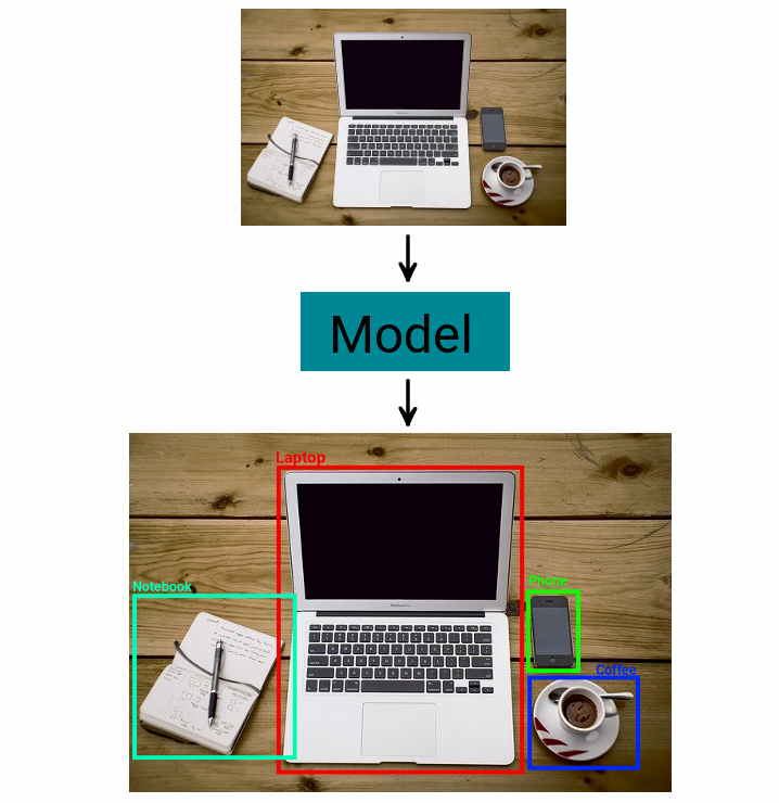
An image is fed to an object detection model which finds and labels the objects of interest in bounding boxes
Baseline approach used for comparison: Faster R-CNN
Faster R-CNN is an object detection model which has been refined over the years and which is used as the baseline to compare with in the paper. Let’s try to understand how it works by seeing it’s evolution over different iterations.
R-CNN
It all started with R-CNN:
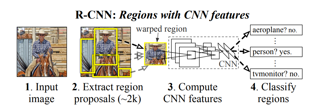
High-level R-CNN architecture, from arXiv:1312.6229v4
Here, a selective search algorithm finds regions of interest in a bottom-up manner. Note that this search algorithm is fixed and not learned during training. Each region proposal is then cropped to a 227x227px square which is separately fed to a CNN backbone which extracts 4096 features. Finally, N different support vector machines are used to determine if the 4096 features are predictive of one of the N classes. To get rid of many duplicate detections, non-maximum suppression is used, i.e. if a region which scores with a low probability for a specific class has a high overlap with another region which scores higher for that class, the first one is removed.
Fast R-CNN
The next iteration from R-CNN is Fast R-CNN with the insight to pass the whole image through the CNN to generate features for the whole image and then use regions of interest on that feature space instead of first making regions of interest and passing many different (repetitive) image parts through the CNN.
This is 9 times faster than R-CNN for training and more than 200 times faster for inference!
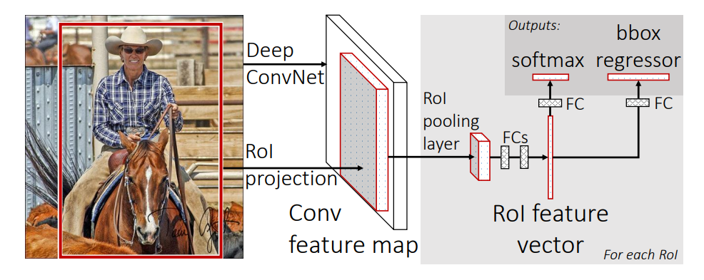
High-level Fast R-CNN architecture, from arXiv:1504.08083v2
So in contrast to R-CNN, there is only one pass through the CNN which is much more efficient given the large overlap of many of the bounding boxes. Afterwards, the region proposals are extracted from the feature space (generated by the CNN) and fed through a region of interest pooling layer and then fully connected layers to finally predict both class probabilites and bounding box regressor offsets. The offsets are used to make the bounding box proposals more accurate.
The region proposals themselves are still generated by using the selective search algorithm.
Faster R-CNN
Next up is Faster R-CNN. It improves on the region selection method. R-CNN and Fast R-CNN used the selective search algorithm to find RoIs on the image in a bottom-up manner. Importantly, this was a pre-defined algorithm which is not improved by the training data. In contrast, Faster R-CNN incorporates the finding of RoIs into a separate neural network, so region finding is learned during training and is not a fixed algorithm anymore. Moreover, it reuses the features generated by the CNN to make region proposals in that feature space.
This is the high-level view of faster R-CNN:
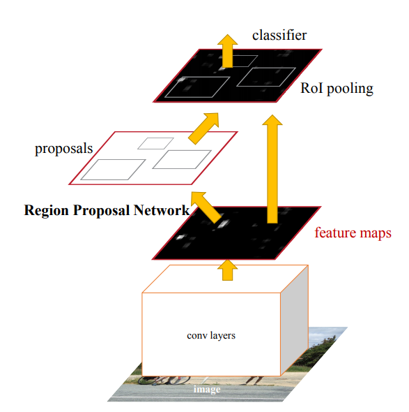
High-level Faster R-CNN architecture, from arXiv:1506.01497v3
The region proposal network (RPN) can be thought of as an attention mechanism which guides the RoI pooling classifier towards the feature areas that are of interest. You can picture the RPN as a sliding window over the image and at each location a set of k anchor boxes (these are hard-coded) are evaluted. For each anchor box at each location, the RPN outputs the probability that it belongs to an object and the bounding box regressor offsets (coordinates to make the bounding box even more indicative of the object of interest). They are using 3 scales and 3 aspect ratios, so 9 different anchor boxes per visual field center location. As before, anchors can overlap significantly, so non-maximum suppression is used on the proposals generated by the RPN.
The network is trained by first training RPN. Then a fast R-CNN network is trained with those proposals. Then the network is frozen at the shared convolutional layers and the RPN is fine-tuned. In the end, the fast R-CNN network is fine-tuned while the shared convolutions are frozen.
Transformer approach of this paper
I hope you gained some insight into the approaches which have been used for object detection so far. The transformer paper wants to get rid of many of the hard-coded / complicated steps needed previously. In particular, it wants to directly predict object boundaries from the image without having specialized, hard-coded anchor boxes or using non-maximum suppression to reduce duplicates. Rather, given an image, it is expected to directly predict bounding boxes with class labels of any size. To do so, an encoder-decoder transformer architecture is devised.
The current methods don’t directly predict object bounding boxes and their classes, but rather have knowledge in terms of anchors built into the design of the system. This limits the detection capabilities, because the objects need to roughly fit those pre-defined anchors. Moreover, they predict many duplicates which are then pruned using non-maximum suppression.
In contrast, the paper of Carion et al. attempts to directly make those predictions without having to deal with many duplicates.
The architecture
In this approach, first a CNN backbone is used to extract features of the image. Those features are fed to an encoder-decoder transformer module which directly outputs object bounding box predictions. If you need a quick reminder of how a transformer works, check out this great illustration by Jay Alammar. To match those predictions with the ground truth labels, a bipartite matching loss is used. This bipartite matching is done using the so-called Hungarian algorithm. They call their model DEtection TRansformer (DETR).
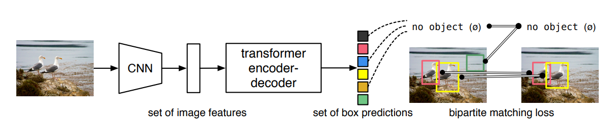
High-level DETR architecture, from arXiv:2005.12872v3
The idea of using a transformer here is that the transformer can use it’s self-attention mechanism to get rid of duplicate predictions. The transformer approach here uses a parallel transformer, i.e. all objects are predicted in parallel rather than having a sequential prediction as often done in natural language processing where the generation of the next word influences the word generated thereafter etc.
One caveat is that the learning process is rather long and you need a good pre-trained backbone suitable to your task as otherwise the training is not very stable. Another one is that the number of predictions is fixed size, so you should set it higher than the expected highest number of objects in your images.
The loss
So what is this bipartite matching loss? It matches predictions to the ground truth. The transformer can output the object bounding boxes in any order. For example if there is a computer, a cell phone and a pen in an image, it doesn’t matter whether the first prediction is the computer or the second prediction is the computer. However, we don’t want to compare the computer prediction to the pen ground truth label. So the bipartite matching loss tries to find the best match between the predictions and the labels.
DETR makes N predictions per image (this is a fixed hyperparameter), but of course N has to be larger than the expected objects in the image. Let’s say the ground truth of an image has M objects where M « N. Then to have a bipartite match, we add (M-N) entries to M which are “no-object”, so that the number in the ground truth and the predictions is of the same size.
The bipartite matching algorithm then finds the best match between the ground truth and the predictions which minimizes the error between them. The error between them takes both the class as well as the similarity of the bounding boxes into account.
Then for all pairs found, the actual loss is a linear combination of the negative log-likelihood for the class prediction and the loss for the box prediction. Importantly, the non-object ground truth values are down-weighted by a factor of 10 to account for class imbalance. The loss for the box prediction in turn is a combination of the l1 loss and the generalized intersection over union loss to make it scale invariant.
Architecture details
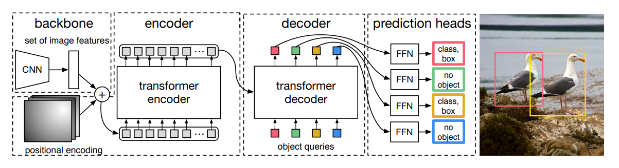
DETR architecture details, from arXiv:2005.12872v3
The image is fed through the CNN to get a feature representation which is of smaller spatial but larger channel dimensionality, e.g. 3x512x512 input image gets transformed to 2048x8x8. Then another 1x1 convolution is applied to reduce the channel dimensions further and the spatial dimensions are flattened as the transformer expects a sequence. So going with the example the 2048x8x8 will be mapped to 256x8x8 using the 1x1 convolution for channel reduction. Then the spatial dimensions (8x8) get flattened out to 8x8=64 and the channels are flipped, so 64x1x256 is finally fed into the transformer. If your image is sized 3x1024x1024, then 256x1x256 will be fed into the transformer.
Like in language transformers, so-called positional encodings are added to the input of the encoder (here: the image features). This is, so the transformer can take advantage of the relative spatial arrangement of the parts provided to it, so it knows which image feature is close to which other one. In this paper, they keep those positional encodings fixed, but you can also make them trainable parameters.
Similary, so-called object queries are added to the decoder. In this case these are indicative of the N predictions we want the decoder to generate, so we pass exactly N object queries to it. The object queries are learnable parameters and adjusted during training. They are fixed at inference time. In the paper, they also show that the object queries are not class specific by making inference on an image with many copies of the same object which gets well detected.
The final N embeddings generated by the transformer are passed to a shared feed forward network (FFN) which has two heads. One head predicts the class (or no-object) and the other head predicts the 4 bounding box coordinates if the class is of an object.
Summary
This is a very interesting approach for object detection and given the large diversity of transformers used for natural language problems, I predict we will see a lot more of these approaches applied to vision problems as well.
The paper proposes DETR which uses a CNN backbone to extract features from images and then feeds them into a transformer which transforms them to a fixed number N of object prediction embeddings. These embeddings are finally passed to a feedforward network with two heads where one head outputs the object class and the other head outputs the 4 bounding box coordinates for each object prediction embedding.
To train this, the best match between the predictions and the ground truth labels is determined using the Hungarian algorithm and based on this match, the loss is a linear combination of the class error and the bounding box error.
Overall, the speed and accuracy of the Faster R-CNN baseline is reached while not needing the custom hard-coded things like non-maximum suppression and fixed anchor boxes.
One important observation is that while the accuracy matches other object detection methods, it performs worse on smaller objects, but better on larger objects. Presumably, the better performance to larger ones is because of the possibility to attend more globally to the image. The worse performance on smaller objects is an open research question.
References
- R-CNN paper by Ross Girshick, Jeff Donahue, Trevor Darrell, Jitendra Malik: Rich feature hierarchies for accurate object detection and semantic segmentation
- Fast R-CNN paper by Ross Girshick: Fast R-CNN
- Faster R-CNN paper by Shaoqing Ren, Kaiming He, Ross Girshick, Jian Sun: Faster R-CNN: Towards Real-Time Object Detection with Region Proposal Networks
- DETR paper by Nicolas Carion, Francisco Massa, Gabriel Synnaeve, Nicolas Usunier, Alexander Kirillov, Sergey Zagoruyko: End-to-End Object Detection with Transformers
machinelearning deeplearning paper objectdetection transformer computervision
Machine Learning Deep Learning Papers
2185 Words
August 30, 2020