7 minutes
Depthwise Separable Convolutions in PyTorch
In many neural network architectures like MobileNets, depthwise separable convolutions are used instead of regular convolutions. They have been shown to yield similar performance while being much more efficient in terms of using much less parameters and less floating point operations (FLOPs). Today, we will take a look at the difference of depthwise separable convolutions to standard convolutions and will analyze where the efficiency comes from.
Short recap: standard convolution
In standard convolutions, we are analyzing an input map of height H and width W comprised of C channels.
To do so, we have a squared kernel of size KxK with typical values something like 3x3, 5x5 or 7x7.
Moreover, we also specify how many of such kernel features we want to compute which is the number of output channels O.
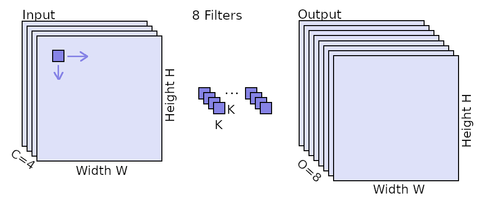
Visual illustration of a convolution. The input feature map is of size WxH and has C channels (here C=4). A kernel of size KxK is moved horizontally and vertically over the input feature map to compute the output for each location. The KxK kernel also covers each of the C channels. There are O of such kernels for each output feature to be computed (here O=8).
The kernels are moved horizontally and vertically over the map and for each location, a value is computed. The value is computed by multiplying the input values with the kernel values and summing them up.
Thus, the number of FLOPs which need to be done for a CNN layer are:
W * H * C * K * K * O, because for output location (W * H) we need to multiply the squared kernel locations (K * K) with the pixels of C channels and do this O times for the O different output features.
The number of learnable parameters in the CNN consequently are: C * K * K * O.
General idea of a depthwise separable convolution
The idea of depthwise separable convolutions is to disentangle the spatial (image height and width) interactions from the channel interactions (e.g. colors). As we have seen above, the standard convolution applies this all together by multiplying values over both several spatial pixels, but also over all the channels.
To separate this, in depthwise separable convolutions, we first use a convolution that is only spatial and independent of channels. In practice, this means that we have an independent convolution per channel. Afterwards we have maps that model the spatial interactions independently of channels, so we apply another convolution that then models the channel interactions. This second operation is often called a pointwise convolution, because it uses a kernel of size 1x1, so models no spatial interactions, but only works on single ‘points’.
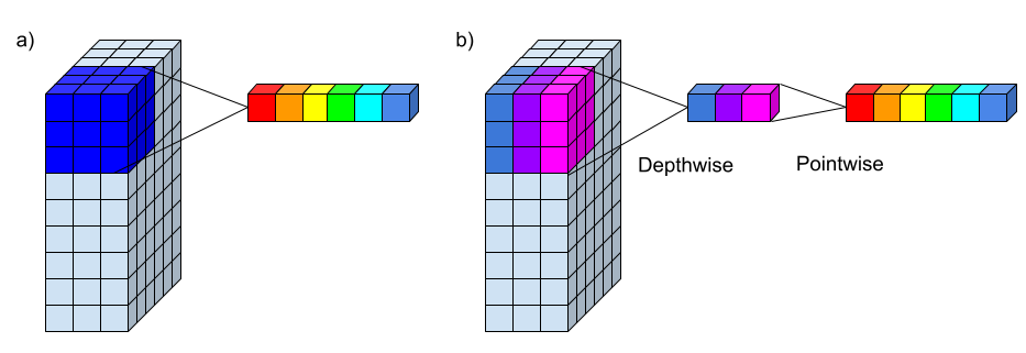
Comparison of a normal convolution and a depthwise separable convolution. a) Standard convolution with a 3x3 kernel and 3 input channels. The projection of one value is shown from the 3x3x3 (dark blue) input values to 6 colorful outputs which would be 6 output channels. b) Depthwise separable convolution with a 3x3 kernel and 3 input channels. First a depthwise convolution projects 3x3 pixels of each input channel to one corresponding output pixel (matching colors). Then a pointwise convolution uses these 3 output pixels to determine the 6 final output pixels.
What’s great about separating these parts?
You save a lot of parameters!
Let’s take a look at both parts independently first.
Depthwise convolution
The depthwise convolution unlike the standard convolution acts only on a single channel of the input map at a time. So for each channel, we need to compute W * H * 1 * K * K FLOPs.
As we have C channels, this sums to W * H * C * K * K FLOPs. The result is a map of C * W * H just like our input map.
In practice, a depthwise convolution is done by using the grouping operation where the number of groups is simply the number of channels (for more info on convolutional grouping, check my article Pyramidal Convolution: Rethinking Convolutional Neural Networks for Visual Recognition).
Pointwise convolution
The second step is the pointwise convolution where we are now using 1 x 1 kernels to have no spatial, but cross-channel interaction.
And we want to map to O output channels, so we need O of these 1 x 1 kernels, so this gives us W * H * C * O FLOPs.
Total operations
Now let’s add the depthwise and the pointwise convolution together: W * H * C * K * K + W * H * C * O = W * H * C * (O + K * K).
Note the difference to the standard convolution: here we have (O + K * K) as a factor instead of O * K * K in the standard convolution.
Let’s say K = 3 and O = 64, then (O + K * K) = 73, but O * K * K = 576.
So for this example, the standard convolution has about 8 times as many multiplications to be calculated!
Total parameters
It’s not only less operations, but also less parameters.
The standard convolution has C * K * K * O learnable parameters as the kernel K * K needs to be learned for all the input channels C and the output channels O.
In contrast, depthwise separable convolution has C * K * K learnable parameters for the depthwise convolution and C * O parameters for the pointwise convolution.
Together, that’s C * (K * K + O) parameters which is again about 8 times less than the standard convolution (for K = 3 and O = 64).
Implementation in PyTorch
We’ll use a standard convolution and then show how to transform this into a depthwise separable convolution in PyTorch. To make sure that it’s functionally the same, we’ll assert that the output shape of the standard convolution is the same as that of the depthwise separable convolution. Of course, we also check the numbers of parameters which we are using.
from torch.nn import Conv2d

conv = Conv2d(in_channels=10, out_channels=32, kernel_size=3)
params = sum(p.numel() for p in conv.parameters() if p.requires_grad)

x = torch.rand(5, 10, 50, 50)
out = conv(x)

depth_conv = Conv2d(in_channels=10, out_channels=10, kernel_size=3, groups=10)
point_conv = Conv2d(in_channels=10, out_channels=32, kernel_size=1)

depthwise_separable_conv = torch.nn.Sequential(depth_conv, point_conv)
params_depthwise = sum(p.numel() for p in depthwise_separable_conv.parameters() if p.requires_grad)

out_depthwise = depthwise_separable_conv(x)

print(f"The standard convolution uses {params} parameters.")
print(f"The depthwise separable convolution uses {params_depthwise} parameters.")

assert out.shape == out_depthwise.shape, "Size mismatch"
Generated output:
The standard convolution uses 2912 parameters.
The depthwise separable convolution uses 452 parameters.
As you can see it’s super easy to implement and can save you a lot of parameters. You simply change the standard convolution to have the same number of out_channels as in_channels (here: 10) and also add the groups parameter which you set to the same value as well. This takes care of our spatial interactions and the groups separates the channels from each other. Then the pointwise convolution is just a convolution mapping the in_channels to the out_channels we had before (here: 32) using a kernel of size 1.
To bind them together, you can use the torch.nn.Sequential, so they are executed one after the other as a bundled module.
Summary
In this blog post, we looked at depthwise separable convolutions.
We learned that they disentangle the spatial and channel interactions that are mixed in a standard convolution.
To do so, a depthwise separable convolution is the combination of a depthwise convolution and a pointwise convolution.
The depthwise convolution maps the spatial relations, but doesn’t interact between channels. Then the pointwise convolution takes the output of the depthwise convolution and models the channel interactions, but keeps a kernel of size 1, so has no further spatial interactions.
The advantage is that we save a lot of parameters and a lot of FLOPs, so overall, the operation is faster and needs less memory.
In practice, it has been shown that depthwise separable convolutions only lead to a minimal performance hit compared to standard convolutions, but drastically reduce the computational needs.
That’s why they are a perfect fit for MobileNetworks where the speed and memory usage is essential.
machinelearning deeplearning convolution pytorch
Machine Learning Deep Learning Papers
1371 Words
February 06, 2021