9 minutes
Pyramidal Convolution: Rethinking Convolutional Neural Networks for Visual Recognition
Today’s paper: Pyramidal Convolution by Duta et al.
This is the third paper of the new series Deep Learning Papers visualized and it’s about using convolutions in a pyramidal style to capture information of different magnifications from an image.
The authors show how a pyramidal convolution can be constructed and apply it to several problems in the visual domain.
What’s really interesting is that the number of parameters can be kept the same while performance tends to improve.
You can find the original paper of Duta et al. on arxiv.
The idea of using convolutional neural networks (CNN) is a success story of biologically inspired ideas from the field of neuroscience which had a real impact in the machine learning world. The visual cortex has cells with small receptive fields which respond to only a restricted area of the visual field. Many of those cells with similar behavior are covering the entire visual field. Thus, the idea came up to reduce the parameters of a fully connected neural network to only a small kernel which is then slid over the entire image to do the same computation again and again.
With enough GPU compute power, Krizhevsky et al. won the ImageNet challenge in 2012 by a large margin with a deep CNN. This led to very high interest in the field in the following years and many think of this as the beginning of the “cambrian explosion” in deep learning.
Duta et al. note that many deep learning architectures nowadays use many CNN layers with sometimes different kernel sizes and some architectures also have several pathways combining the input image at different resolutions. However, so far, this is architected in network pathways, so the idea of the authors is to directly build a pyramidal multi-resolution analysis into the convolution operation. This is what they call Pyramidal Convolution and we will look at it in detail in this post.
Short recap: standard convolution
In a standard (non pyramidal) convolution, we are analyzing an input map of height H and width W comprised of C channels.
To do so, we have a squared kernel of size KxK with typical values something like 3x3, 5x5 or 7x7.
Moreover, we also specify how many of such kernel features we want to compute which is the number of output channels O.
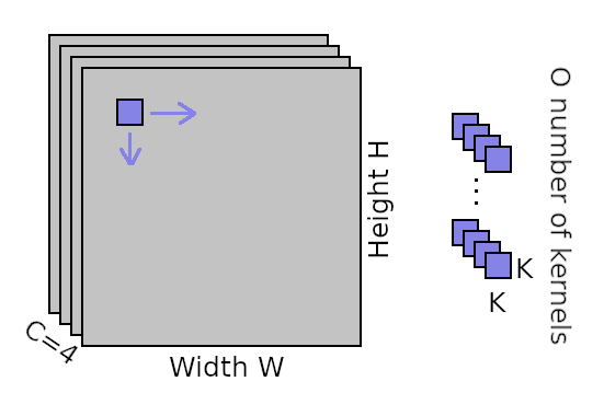
Visual illustration of a convolution. The input feature map is of size WxH and has C channels (here C=4). A kernel of size KxK is moved horizontally and vertically over the input feature map to compute the output for each location. The KxK kernel also covers each of the C channels. There are O of such kernels for each output feature to be computed.
The kernels are moved horizontally and vertically over the map and for each location, a value is computed. The value is computed by multiplying the input values with the kernel values and summing them up.
Thus, the number of floating point operations which need to be done for a CNN layer are:
W * H * C * K * K * O, because for each pixel location (W * H) we need to multiply the squared kernel locations (K * K) with the pixels of C channels and do this O times for the O different output features.
The number of learnable parameters in the CNN consequently are: C * K * K * O.
Pyramidal Convolution
The pyramid idea comes from the fact that in image processing, it is often beneficial to have the input image at different scales, so the image can be analyzed on larger and smaller scales looking for more local / smaller features and for more global / larger features.
The idea of Duta et al. is to put this idea into the convolution by using approximately the same number of parameters as a standard CNN does, but design the parameters so that they cover different spatial aspects of the input map.
This is achieved by analyzing the input map with kernels of different sizes.
The computational challenge
Let’s assume for a minute that we have an input map with 200 x 200 pixels and 64 channels. Also consider we are using a standard convolution with 128 output channels and a kernel size of 3x3.
Then, the number of parameters are: 64 * 3 * 3 * 128 = 73728.
What if we used a kernel of size 5x5? The number of parameters would increase a lot: 64 * 5 * 5 * 128 = 204800.
Now, if we even combined both of these scales and used both the filter of 3x3 and the filter of 5x5, we’d end up with 278528 parameters which is about 4 times as much as we started out with.
Going this route, our network would quickly get very slow to train.
That’s why we need to somehow restrict the number of parameters to make them comparable to the default convolution case.
Grouped convolutions
The authors refer to the idea of grouped convolutions where we split the number of input channels and the number of output channels into groups and then do the convolution only between members of the groups. This has been shown to lead to some interesting computational gains by itself while restricting the computational needs as already reported in the original AlexNet paper.
The larger our kernel is, the higher the number of parameters, so we should have less feature depth / input channels dedicated to the larger kernels. And this is exactly what can be achieved with grouped convolutions:
Let’s consider the case of using the kernel of size 5x5, but now split this into 2 groups which means we split the 64 input channels into 2 groups of 32 channels each and the output feature maps of 128 into 2 groups of 64 outputs.
Then for each group, the number of parameters is: 32 * 5 * 5 * 64 = 51200. We have this 2 times now (once for each group), so the total parameters are 102400 which is only half as much as without the grouping!
This is how the pyramid comes about: for the smallest kernel, we have the least amount of parameters, so it can get away without using much grouping, but as we increase the kernel size, we walk the pyramid upwards and in turn increase the grouping to balance off the spatial parameter increase.
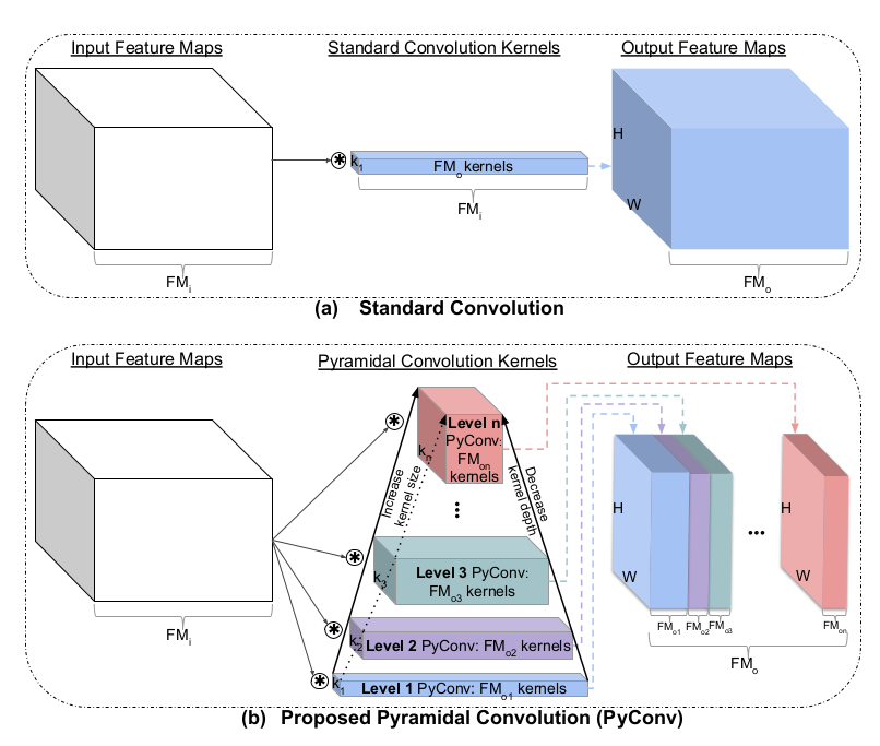
Figure taken from arXiv:2006.11538. a) here refers to the standard convolution where they use FM_i instead of C and FM_o instead of O. b) Pyramidal convolution illustration. You can see that towards the top of the pyramid, the kernel size is increased while the kernel depth is decreased (i.e. the number of groups is increased).
So if we want to use both the kernel size 3 and 5 and have 128 output channels, we divide the output channels on both of these kernels, so the kernel 3 computes 64 outputs and the kernel 5 also computes 64 outputs. But also since kernel 5 is larger, we’ll use 4 groups here.
Then the number of parameters will be:
64 * 3 * 3 * 64 = 36864 for the 3x3 kernel and 16 * 5 * 5 * 16 = 6400 for each of the 4 groups for the 5x5 kernel. The total amount of parameters is thus 36864 + 4 * 6400 = 62464, so even less parameters then the full 3x3 kernel convolution before.
Applying Pyramidal Convolutions
The authors show how to apply pyramidal convolutions into ResNets by replacing the residual blocks with pyramidal residual blocks which are constructed as follows:
First a 1x1 bottleneck convolution is applied which reduces the incoming channels to a defined number like 64 or 128. It’s followed by BatchNorm and ReLU activation function and then a pyramidal convolution which is constructed as described above, so has small kernels without groups at the bottom and then increases the kernel size and the number of groups going upwards in the pyramid.
For example, for 64 channels, they use at the base a 3x3 convolution without grouping which produces 16 of the output channels. Going up the pyramid, a 5x5 convolution with 4 groups also produces 16 output channels. Then a 7x7 convolution with 8 groups produces another 16 output channels. Finally, a 9x9 kernel with 16 groups (i.e. 4 input channels are connected to a single output channel) produces the remaining 16 output groups. So in total, the Pyramidal convolution produces 64 output channels with 16 channels for each kernel size.
After the Pyramidal convolution and another BatchNorm + ReLU, another 1x1 convolution is used again to increase the number of channels to the original input channels, again followed by BatchNorm and ReLU activation function.
This concludes the residual bottleneck pyramidal block which is used several times replacing the original ResNet blocks.
Doing so, the number of parameters and FLOPs is even reduced a bit, but the fun thing is that the overall performance is improved. For example on the ImageNet recognition task, the top 1% error rate drops by almost 2% compared to the ResNet baseline.
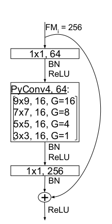
Figure taken from arXiv:2006.11538. Illustration of the residual bottleneck pyramidal block. Notation is KxK, O, # of groups G. BN is BatchNorm.
You can check out their implementation on Github.
Summary
The paper proposes pyramidal convolutions to capture image information for different magnifications. To make it computationally feasible to have several also large kernels, they use the idea of grouped convolutions to reduce the number of parameters for larger kernels. Doing so, a pyramid can be constructed which has small kernels with no / little grouping at the base and as the kernel size increases, so does the grouping.
They go on to show that having this information from several resolutions tends to help in many visual problems when applying it to image recognition, object detection or image segmentation (I have only reported some of those findings in this blog post, please refer to the paper for more details).
Overall, I think it’s a great idea to capture image information at several spatial resolutions directly from convolutions and will definitely try this out.
References
- Pyramidal Convolution paper by Ionut Cosmin Duta, Li Liu, Fan Zhu and Ling Shao: Pyramidal Convolution: Rethinking Convolutional Neural Networks for Visual Recognition
- AlexNet paper by Alex Krizhevsky, Ilya Sutskever and Geoffrey E. Hinton: ImageNet Classification with Deep Convolutional Neural Networks
machinelearning deeplearning paper objectdetection convolution
Machine Learning Deep Learning Papers
1733 Words
November 29, 2020