Eigenvectors and eigenvalues in machine learning :: Päpper's Machine Learning Blog — This blog features state of the art applications in machine learning with a lot of PyTorch samples and deep learning code. You will learn about neural network optimization and potential insights for artificial intelligence for example in the medical domain.

As a data scientist, you are dealing a lot with linear algebra and in particular the multiplication of matrices. Important properties of a matrix are its eigenvalues and corresponding eigenvectors.

So let’s explore those a bit to get a better intuition of what they tell you about the transformation.

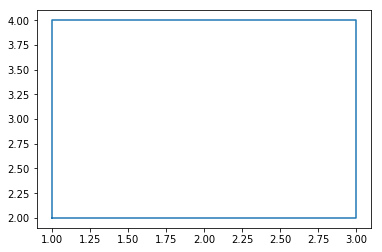
We will just need numpy and a plotting library and create a set of points that make up a rectangle (5 points, so they are visually connected in the plot):

import numpy as np
import matplotlib.pyplot as plt

matrix = np.array([[2.0, 1.0],[1.0, 2.0]])
points = np.array([[1.0, 1.0, 3.0, 3.0, 1.0], [2.0, 4.0, 4.0, 2.0, 2.0]])

plt.plot(points[0], points[1])
plt.show()

png

Applying the matrix to the points

To apply the matrix to our points we can simply use np.matmul(matrix, points) which will do this in a vectorized (i.e. fast) way. We’ll plot the before and after and abstract this to a function which we can reuse later:

def plot_before_after(points, matrix, value_range=None):
    fig, ax = plt.subplots(figsize=(5, 5))
    if value_range is not None:
        ax.set_xlim(value_range[0], value_range[1])
        ax.set_ylim(value_range[0], value_range[1])
    ax.plot(points[0], points[1], 'bo-')
    transformed = np.matmul(matrix, points)
    ax.plot(transformed[0], transformed[1], 'rx--')
    plt.legend(labels=['before', 'after'])
    plt.show()

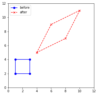
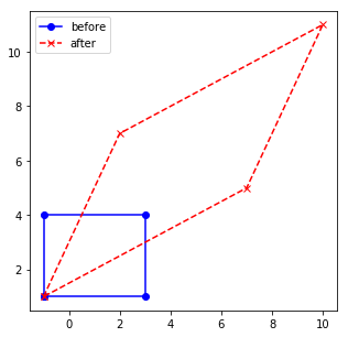
plot_before_after(points, matrix, value_range=[0, 12])

png

Getting the eigenvalues and eigenvectors

Pretty cool! We can see that our blue rectangle was transformed into an enlarged red parallelogram. So let’s find out how the eigenvalues and eigenvectors played along here. Luckily the function np.linalg.eig(matrix) returns us both the eigenvalues as well as eigenvectors:

eigenvalues, eigenvectors = np.linalg.eig(matrix)
eigenvalues, eigenvectors

(array([3., 1.]), array([[ 0.70710678, -0.70710678],
        [ 0.70710678,  0.70710678]]))

Alright, so we find that we have two eigenvalues in this matrix: 3 and 1. The eigenvectors are (0.707, 0.707) and (-0.707, 0.707) respectively.

We can verify that this is true, because to be an eigenvector of a matrix, the result of multiplying the vector with the matrix has to be the scaled vector again. The scaling factor is exactly the eigenvalue, so the multiplication with the matrix should be the same as multiplying the vector directly by its eigenvalue:

matrix_times_vector = np.matmul(matrix, eigenvectors[:,0])
vector_scaled_by_eigenvalue = eigenvalues[0] * eigenvectors[:, 0]
print(matrix_times_vector, vector_scaled_by_eigenvalue)

[2.12132034 2.12132034] [2.12132034 2.12132034]

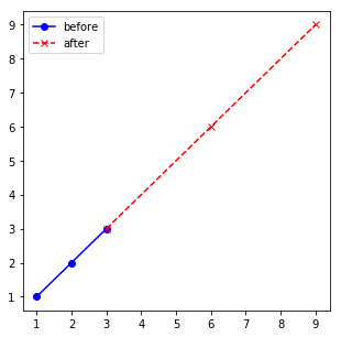
So what does this tell us now? This means that our matrix scales points which are in the vector axis (0.707, 0.707) by a factor of 3 while not changing their orientation in space. And this will happen for each point which is on the line which is spanned up by the vector. We can clearly see this when we take some of those points and apply the matrix to it. The original points (blue) as well as their images (red) are on the same line:

eigenvector_points = np.array([[1, 2, 3], [1, 2, 3]])
plot_before_after(eigenvector_points, matrix)

png

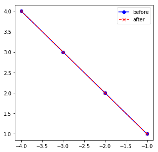
In contrast, points which are on the line (-1, 1), they are scaled with the eigenvalue 1, so in fact they don’t change at all (red and blue points are on top of each other):

eigenvector_points2 = np.array([[-1, -2, -3, -4], [1, 2, 3, 4]])
plot_before_after(eigenvector_points2, matrix)

png

Now going back to the original question: what does this tell us about the matrix operation? Well, we learned that in the right upward facing direction, data will be scaled by a factor of 3, while data which is in the left upward facing direction, the scaling will be much lower:

points = np.array([[-1.0, -1.0, 3.0, 3.0, -1.0], [1.0, 4.0, 4.0, 1.0, 1.0]])
plot_before_after(points, matrix)

png

Furthermore, the knowledge about eigenvectors and eigenvalues can help us out in very important aspects. Consider this “weird matrix”:

weird_matrix = np.array([[2.0, 1.0], [0.0, 0.0]])
plot_before_after(points, weird_matrix)

png

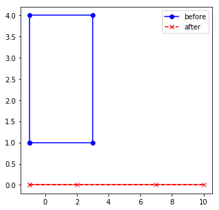
It collapses our rectangle to a straight line. Hmm, what is going on? Let’t take a look at the eigenvalues:

np.linalg.eig(weird_matrix)

(array([2., 0.]), array([[ 1.        , -0.4472136 ],
        [ 0.        ,  0.89442719]]))

One of the eigenvalues turns out to be 0. If an eigenvalue is 0, then all points in that dimension are reduced to 0. So this is what is happening here: our 2-dimensional rectangle gets projected to a one-dimensional line. Knowing the eigenvalues thus can tell you what kind of projection your matrix does.

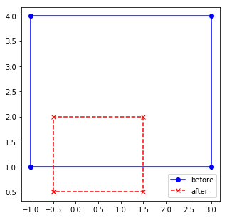
One last look at another matrix which has eigenvalues that are smaller than 1. In this case, the original space (blue) gets shrinked down:

new_matrix = np.array([[0.5, 0], [0, 0.5]])

plot_before_after(points, new_matrix)

png

Summary

We took a look at the eigenvectors and eigenvalues of several matrices. Inspecting the eigenvalues we can learn:

Small eigenvalues (smaller than 1.) indicate that our data points will be smaller after the transform in the direction of the corresponding eigenvector
Large eigenvalues (larger than 1.) indicate that our data points will be larger after the transform in the direction of the corresponding eigenvector
When there are eigenvalues with 0. this indicates that dimensionality will be reduced, so a smaller matrix could be used to achieve the same transform.