As a developer, you are often asked how long it will take to program a certain module or feature for some software project. This can be annoying at times, so let’s make it more fun! In this post, we are going to use a data science approach to get up with better estimates. The whole post will be covered by simple Python code, which you can easily use for your own estimates.

Our estimate for the super-awesome mega feature

For the sake of this post, we want to estimate the super-awesome mega feature. To make a good estimate, it is wise to separate it into different work chunks rather than just coming up with a number. For each work chunk, we usually have some idea from our experience of how long this is gonna take:

• We think that we will need about 5 hours for the initial setup
• We speculate that the development itself will take around 10 hours
• We propose to spend 5 hours on testing afterwards

Now, we could just take the sum of the chunks: 5 + 10 + 5 = 20 hours. This would give us a good first idea, but how confident are we that we get the job done in 20 hours?

Let’s try to make the estimate better by assigning confidence scores and ranges to our chunks of work:

• The initial setup is fairly easy to estimate, so we will say we are 95% confident that it is 4-6 hours
• The development of the super-awesome mega feature is rather unsure as often when developing we identify issues we didn’t think of before etc, so we will say this is 60% sure that it is between 8-16 hours
• Given the specs of the feature, testing shouldn’t be too difficult. However, we cannot be as sure as for the setup, so we will assign it a 90% confidence score for an estimate of 4-10 hours.

To deal with our estimate, let’s turn it to code:

A named tuple for our Estimate

We will create a representation for our estimates by creating a named tuple called Estimate. It has three properties: low, high and confidence. Low and high represent our estimate boundaries and confidence our confidence percentage.

import numpy as np
from scipy import stats
import matplotlib.pyplot as plt
%matplotlib inline

import collections

Estimate = collections.namedtuple('Estimate', 'low, high, confidence')

setup = Estimate(low=4, high=6, confidence=95)
development = Estimate(low=8, high=16, confidence=60)
testing = Estimate(low=4, high=10, confidence=90)

Confidence intervals

In statistics, a normal distribution or Gaussian distribution is one of the most used distributions. It has a mean which is the most probable value and a standard deviation indicating how far the values spread from the mean. If the standard deviation is small, then the distribution is peaky and narrow. If the standard deviation is large, the distribution is broad and wide.

The confidence interval indicates an area around the mean in which randomly drawn values of the distribution should fall in a certain percentage of times. For example, if we take a 95% confidence interval around the mean in a normal distribution that refers to 1.96 standard deviations around the mean. And if we draw 100 random values from the distribution, 95 should on average lie within that interval. Why the 1.96 I hear you ask? Well, that is a property of the normal distribution given its cumulutive probability distribution and you can read off these values in so-called z-tables, e.g. look here.

Given that we estimated a confidence value for our chunks of work, we want to use confidence intervals to put our estimates into probability distributions. The mean of the distribution is easy as we just add the low and high together and divide it by 2. But what about the standard deviation? Ideally, given our confidence estimate, we could model it such that the confidence interval covers our low and high value. That is: mean - x = low and mean + x = high. How to get x? Well, if we have a confidence interval, then x is the z-score multiplied with the standard deviation.

mean + (z * std) = high
<-> z * std = high - mean
<-> std = (high - mean) / z

As we can read the z score from a z-table, we can thus use it to calculate a proper standard deviation for our distribution!

def get_confidence_interval(confidence):
    if confidence == 95:
        return 1.96
    elif confidence == 90:
        return 1.65
    elif confidence == 80:
        return 1.28
    elif confidence == 70:
        return 1.04
    elif confidence == 60:
        return 0.84
    else:
        raise(ValueError("You specified a confidence which is not yet defined here. You can add it by reading it from a z-table."))

def get_distribution(estimate):
    confidence_interval = get_confidence_interval(estimate.confidence)
    mean = (estimate.high + estimate.low) / 2
    std_deviation = (estimate.high - mean) / confidence_interval
    
    return stats.norm(loc=mean, scale=std_deviation)

Monte Carlo estimate

We are at the point that we know how to represent our chunks of work as probability distributions over hours of work. From each probability distribution, we can randomly draw numbers and add them together to get to a final estimate. If we repeat this process many times, we should get a good idea of the real amount of time it will take us. This is called a Monte Carlo estimate. We simply run a large amount of experiments during which we sample from our distributions, we sum the results up and divide by the number of experiments.

def plot_estimate(estimates, num_experiments = 100000):
    distributions = [get_distribution(estimate) for estimate in estimates]
    draws = [distribution.rvs(num_experiments) for distribution in distributions]
   
    plt.subplot(2,2,1)
    plt.hist(sum(draws), bins=100)
    
    plt.subplot(2,2,2)
    values, base = np.histogram(sum(draws), bins=100)
    cumulative = np.cumsum(values / num_experiments)
    plt.plot(base[:-1], cumulative, c='blue')
    
    print("On average, it takes {:.2f} hours.".format(np.sum(sum(draws)) / num_experiments))

plot_estimate([setup, development, testing])

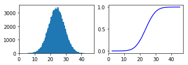
On average, it takes 24.04 hours.

The result

As we can see, we get to a rough estimate of 24 hours which is a much better estimate than our initial guess. Moreover, we can get much more information from our graphs.

We can now look at the distribution which is our histogram on the left. This is the representation of all our experiments and the number of experiments which resulted in a certain number of hours. The average of all experiments was 24.04 hours which you can also see in the left graph as the highest peak in the distribution is around x = 24.

Moreover, we plot the cumulative distribution function on the right side. It represents the probability of the number of hours being below a certain value which you can read on the x-axis. We can now also say that we can be rather confident that it should take us not more than 30 hours as the probability is around 90% for taking <= 30 hours.