8 minutes
Debugging Tensorflow

Debugging Tensorflow
Today, I am going to explore different ways to debug Tensorflow which can be a bit cumbersome at times. However, there are a few good possibilities that I know of to get more insight into the inner workings of Tensorflow.
It’s a little more complicated than regular debugging like say in PyTorch where you can use an IDE like PyCharm and simply set breakpoints in your code to stop and inspect what’s going on.
This is because Tensorflow separates the creation of a computation graph and the execution of data flowing through the graph in a session.
A simple example: MNIST
MNIST is a classic machine learning dataset which consists of small hand-written images of the numbers 0-9 and their respective labels. The goal when training MNIST is to predict the digits of images which the algorithm hasn’t seen during training.
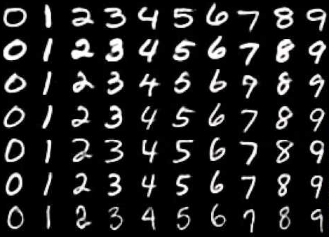
MNIST example digits
Let’s first load the data:
import tensorflow as tf
from tensorflow.contrib.learn.python.learn.datasets.mnist import read_data_sets

mnist = read_data_sets("data", one_hot=True, reshape=False, validation_size=0)
Network design in Tensorflow
We will build a very simple solution for MNIST using just a single neuron layer. Note that this can be improved much by using CNNs, but here we are more concerned to have a simple example to debug in Tensorflow.
We flatten the 28x28 pixel images to have a 784-dimensional vector which is multiplied with the weight matrix W to map it to 10 output values and then add the bias b.
To make sure that the 10 output values represent the probabilities of the 10 digits, we apply a softmax activation function which makes sure the output sums to 1.
As our loss function, we are using cross_entropy which we minimize in our GradientDescentOptimizer with a learning rate of 0.005.
tf.reset_default_graph()

X = tf.placeholder(tf.float32, [None, 28, 28, 1], name='input')

W = tf.Variable(tf.zeros([784, 10]), name='weights')
b = tf.Variable(tf.zeros([10]), name='bias')

init = tf.global_variables_initializer()

X_flat = tf.reshape(X, [-1, 784], name='X_flat')

Y_hat = tf.nn.softmax(tf.matmul(X_flat, W) + b, name='Y_hat')

Y = tf.placeholder(tf.float32, [None, 10], name='answers')

cross_entropy = -tf.reduce_sum(Y * tf.log(Y_hat), name='cross_entropy')

is_correct = tf.equal(tf.argmax(Y_hat, 1), tf.argmax(Y, 1), name='is_correct')
accuracy = tf.reduce_mean(tf.cast(is_correct, tf.float32), name='accuracy')

optimizer = tf.train.GradientDescentOptimizer(0.005)
train_step = optimizer.minimize(cross_entropy)
The Tensorflow training loop
In the step above we defined our operations and now we will make sure that actual data flows through them. We run 1000 loops of 100-image batches. Every 100 iterations, we evaluate how the network is doing on the train and the test set.
Note that with this simple approach, we achieve > 90% accuracy on the test set.
sess = tf.Session()
sess.run(init)
test_data = {X: mnist.test.images, Y: mnist.test.labels}

for i in range(1000):
    batch_X, batch_Y = mnist.train.next_batch(100)

    train_data = {X: batch_X, Y: batch_Y}
    sess.run(train_step, feed_dict=train_data)

    if i % 100 == 0:
        train_acc, train_error = sess.run([accuracy, cross_entropy], feed_dict=train_data)

        test_acc, test_error = sess.run([accuracy, cross_entropy], feed_dict=test_data)

        print("Train: acc. {:2.0f}%, error: {:5.2f}            Test: acc. {:2.0f}%, error {:5.2f}".format(train_acc * 100, train_error, test_acc * 100, test_error))

print("\n\n---------- Results ----------")
print("{:2.1f}% accuracy on test data".format(sess.run(accuracy, feed_dict=test_data) * 100))
Train: acc. 37%, error: 178.24 Test: acc. 23%, error 21132.81
Train: acc. 90%, error: 35.84 Test: acc. 89%, error 4025.79
Train: acc. 93%, error: 22.77 Test: acc. 91%, error 3397.53
Train: acc. 96%, error: 17.66 Test: acc. 91%, error 3226.82
Train: acc. 94%, error: 17.74 Test: acc. 91%, error 3165.46
Train: acc. 96%, error: 21.39 Test: acc. 91%, error 3075.05
Train: acc. 96%, error: 18.60 Test: acc. 92%, error 3036.30
Train: acc. 95%, error: 15.80 Test: acc. 91%, error 3089.97
Train: acc. 94%, error: 30.76 Test: acc. 91%, error 3052.03
Train: acc. 95%, error: 15.52 Test: acc. 92%, error 2997.80 \——— Results ———
91.9% accuracy on test data
Debugging with Tensorflow
As we’ve seen, we separated the network creation and the data flow which is what complicates our debugging process a little bit. Let’s say we want to have a look at the probabilities which our network outputs. What can we do?
Using a session run
The first possibility we have is to actually retrieve the probabilities by using sess.run([Y_hat], feed_dict=test_data) to tell Tensorflow to retrieve the probabilities (Y_hat) for us by feeding in our test_data to evaluate on:
probabilities = sess.run([Y_hat], feed_dict=test_data)
print(probabilities)
[array([[3.78640143e-05, 4.72710981e-09, 8.43762464e-05, …, 9.95767593e-01, 2.31660124e-05, 4.51680884e-04], [3.90564528e-05, 1.07444727e-10, 7.70817744e-04, …, 9.36290712e-10, 2.33943933e-06, 3.17476250e-08]], dtype=float32)]
Using tf.Print() / tf.print() for debug operations
In our example, the above mechanism works quite well. We could even incorporate it into our loop and retrieve the probabilities for every run. However, sometimes this doesn’t work as well if you have more complicated models where the thing you are interested in is not a Tensorflow operation which is available to you and might be hidden deep inside some file or model.
An alternative then is to go directly into the file you are interested in and use the tf.Print() operation to make it explicit at that step.
I will illustrate this with Y_hat as well:
Y_hat = tf.nn.softmax(tf.matmul(X_flat, W) + b, name="Y_hat")
Y_hat = tf.Print(Y_hat, [Y_hat], "Y_hat is ", name="Print_Y_hat")

cross_entropy = -tf.reduce_sum(Y * tf.log(Y_hat), name="cross_entropy")
If we run our training loop again, the debug output is printed. However, note a couple of things:
- The output is printed to standard error which doesn’t show in Jupyter notebooks directly. You can see the output in the terminal where you started the Jupyter notebook server!
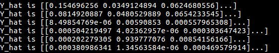
Output from tf.Print() in the terminal
-
Note that you need to use the resulting operation of tf.Print() somewhere, so it is included in the Tensorflow graph. This is the reason, I needed to also redefine cross_entropy here, so it uses the new definition of Y_hat.
-
Starting with Tensorflow 1.12 the function tf.Print() is deprecated. In the future, you should use tf.print() which behaves a little bit differently. Use it like this:
print_op = tf.print("Y_hat is ", Y_hat, output_stream=sys.stdout)
with tf.control_dependencies([print_op]):
    cross_entropy = -tf.reduce_sum(Y * tf.log(Y_hat))
Visualize information using Tensorboard
Using Tensorboard is a great idea to get a better grasp of what is going on inside your network. Besides plotting the Tensorflow graph, it also allows you to plot specific data as you request.
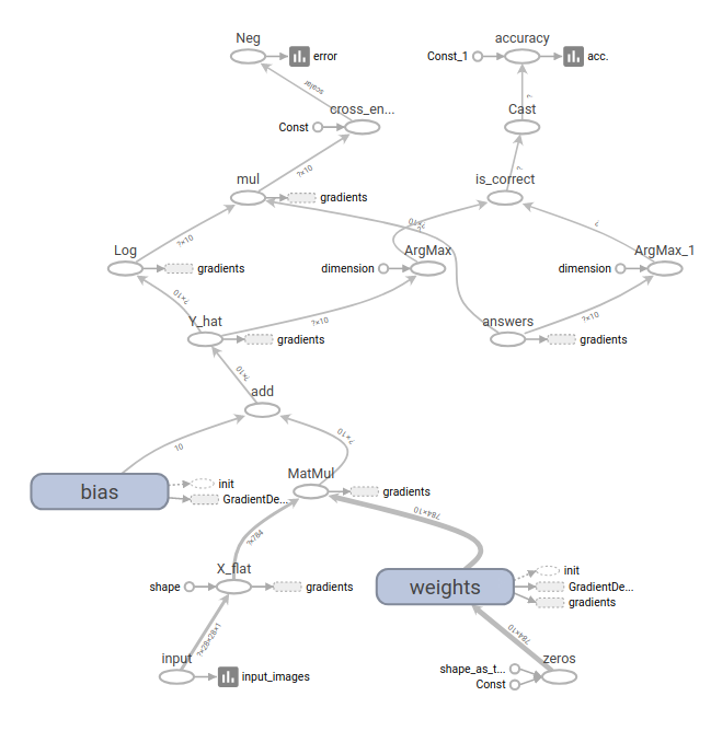
Plot of the network graph in tensorboard
To do so, you will need to create a summary writer which is able to write all your information: writer = tf.summary.FileWriter([logdir], [graph]).
Then, for each piece of information you are interested in, you use tf.summary to create a summary over time.
These are the possible summary operations:
-
tf.summary.scalar: used to write a single scalar-valued tensor like the loss or accuracy value.
-
tf.summary.histogram: used to plot histogram of all the values of a non-scalar tensor. This can be used to plot your weights matrix.
-
tf.summary.image: used to plot images like our input images.
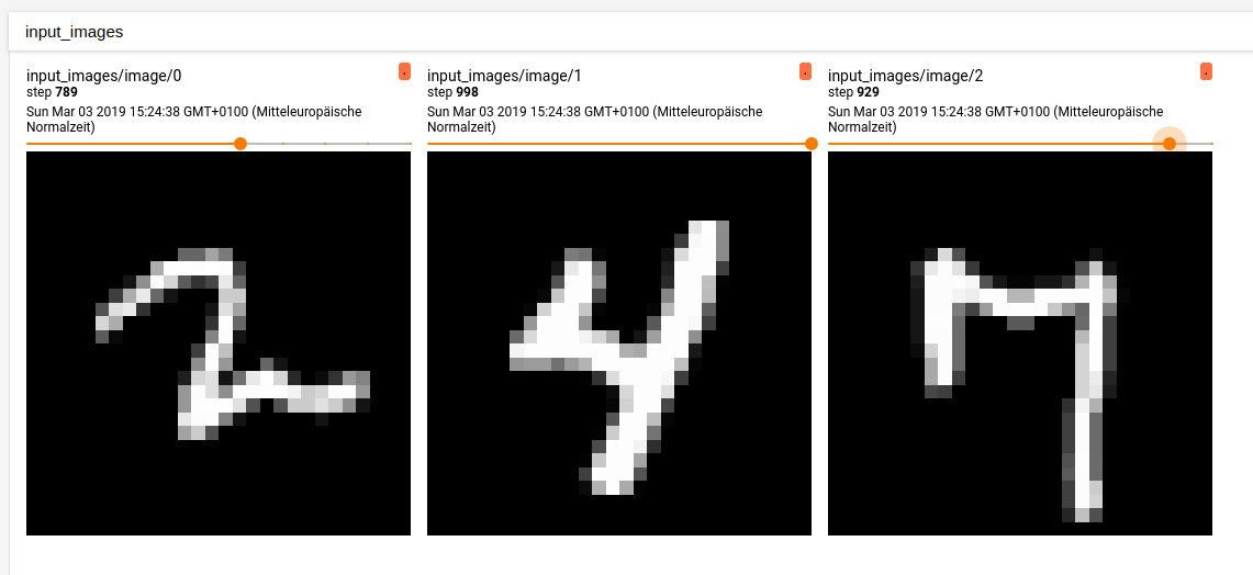
Example output of tensorboard images
Also, we create a summary_operation which then can be fed into the sess.run call to evaluate all summaries instaed of calling each one by itself.
Finally, we write the summary we obtain from sess.run with our file writer: writer.add_summary(summary, i)
sess = tf.Session()
sess.run(init)

tf.summary.scalar('acc.', accuracy)
tf.summary.scalar('error', cross_entropy)
tf.summary.image('input_images', X)
tf.summary.histogram('weights', W)
summary_operation = tf.summary.merge_all()
test_data = {X: mnist.test.images, Y: mnist.test.labels}

writer = tf.summary.FileWriter('mnistlog', sess.graph)

for i in range(1000):
    batch_X, batch_Y = mnist.train.next_batch(100)

    train_data = {X: batch_X, Y: batch_Y}
    _, summary = sess.run([train_step, summary_operation], feed_dict=train_data)

    writer.add_summary(summary, i)

    if i % 100 == 0:
        train_acc, train_error = sess.run([accuracy, cross_entropy], feed_dict=train_data)

        test_acc, test_error = sess.run([accuracy, cross_entropy], feed_dict=test_data)

        print("Train: acc. {:2.0f}%, error: {:5.2f}            Test: acc. {:2.0f}%, error {:5.2f}".format(train_acc * 100, train_error, test_acc * 100, test_error))

print("\n\n---------- Results ----------")
print("{:2.1f}% accuracy on test data".format(sess.run(accuracy, feed_dict=test_data) * 100))
Train: acc. 51%, error: 166.52 Test: acc. 35%, error 20278.74
Train: acc. 84%, error: 42.66 Test: acc. 89%, error 3934.66
Train: acc. 94%, error: 32.13 Test: acc. 90%, error 3470.43
Train: acc. 91%, error: 40.86 Test: acc. 91%, error 3317.01
Train: acc. 88%, error: 36.47 Test: acc. 91%, error 3197.21
Train: acc. 93%, error: 25.72 Test: acc. 92%, error 3081.94
Train: acc. 93%, error: 28.42 Test: acc. 91%, error 3067.98
Train: acc. 94%, error: 28.57 Test: acc. 92%, error 2985.85
Train: acc. 94%, error: 28.29 Test: acc. 92%, error 2944.46
Train: acc. 94%, error: 23.34 Test: acc. 92%, error 2936.88
——— Results ———
92.0% accuracy on test data \
Debugging Tensorflow with Tensorboard
Besides enabling you to output statistics, values, images and more, another exciting option in Tensorboard is that you can use it as a graphical debugging tool as well. To do so, you need to do two things:
a) Start tensorboard with debug operations: tensorboard --logdir log/dir/ --debugger_port 6064
b) Wrap your Tensorflow session in a debug operation: tf_debug.TensorBoardDebugWrapperSession(sess, "URL") - note that you should include the port specified in a)
from tensorflow.python import debug as tf_debug

sess = tf.Session()
sess = tf_debug.TensorBoardDebugWrapperSession(sess, "localhost:6064")
sess.run(init)

for i in range(1000):
    batch_X, batch_Y = mnist.train.next_batch(100)

    train_data = {X: batch_X, Y: batch_Y}
    sess.run(train_step, feed_dict=train_data)

    if i % 100 == 0:
        train_acc, train_error = sess.run([accuracy, cross_entropy], feed_dict=train_data)

        test_acc, test_error = sess.run([accuracy, cross_entropy], feed_dict=test_data)

        print("Train: acc. {:2.0f}%, error: {:5.2f}            Test: acc. {:2.0f}%, error {:5.2f}".format(train_acc * 100, train_error, test_acc * 100, test_error))

print("\n\n---------- Results ----------")
print("{:2.1f}% accuracy on test data".format(sess.run(accuracy, feed_dict=test_data) * 100))
This is how the debugger view looks like. You can use the step button at the lower left side to iterate through your loop:
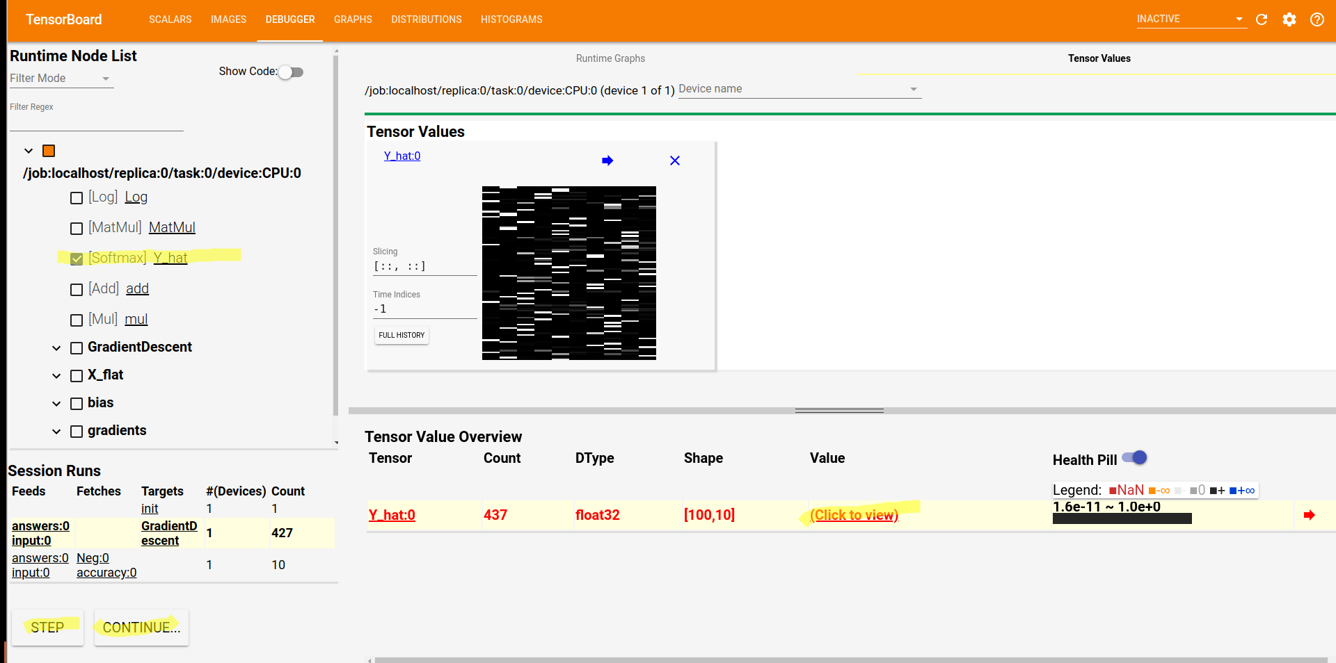
Debug view in Tensorboard.
And here is a comparison of Y_hat at the beginning of training (you can see that it is still unsure about the 10 digits):
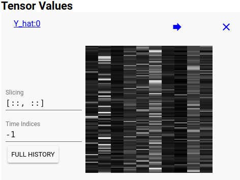
Y_hat at the beginning of training.
And here it is after training (now pretty sure about the digits, so clearer white colors):
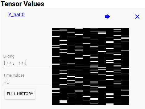
Y_hat at the end of training.