7 minutes
Deep Learning on Medical Images With U-Net

Illustration taken from the U-Net paper
I recently read an interesting paper titled “U-Net: Convolutional Networks for Biomedical Image Segmentation” by Olaf Ronneberger, Philipp Fischer, and Thomas Brox which describes how to handle challenges in image segmentation in biomedical settings which I summarize in this blog post.
Challenges for medical image segmentation
A typical task when confronted with medical images is segmentation. That refers to finding out interesting objects in an image. This could for example be cancer cells on a CT scan. The important aspect here is that you not only want to classify images as cancer / no cancer, but rather you want to localize the indivual pixels of the image as cancer / no cancer.
Therefore, you need both classification as well as localization.
To make things more complicated, you typically don’t have much data. When you use a big dataset such as ImageNet you have plenty of pictures to train on, but medical images are usually much sparser.
It’s just much more costly to obtain the data as there are privacy concerns (you need patients consent to use the data) and you need experts (think doctors) which are able to accurately label the data, so you have the correct localization labels.
Thus, money and time constraints lead to only a low amount of data.
To get around this, the approach taken is to massively augment the data (i.e. generate several images from one image) as illustrated in the next paragraph.
Data augmentation
As the authors train their network on only 30 images, extensive data augmentation is used to generate more data. Especially, they use the following:
- Shifting: shifting the image a few pixels to either side
- Rotations: rotating the image by a few degrees adds robustness for images taken at slightly different angles
- Elastic deformations: 3x3 pixel grid of random displacements with bicubic per-pixel displacements
- Gray value variations: changing the color of the images
The big picture of the U-Net architecture
There are three main parts to the U-Net architecture:
- Down path: The down path is the ‘classical’ convolution path where the image resolution shrinks the deeper into the layers you get while the number of channels increases.
- Up path: The up path is the inverse of the down path to increase the resolution again to be able to handle the localization challenge. This is done by upscaling the image size while reducing the number of channels over time.
- Concatenations: An important aspect of U-Net is the combination of the down path with the up path by using concatenations. By doing so the net can learn to classify and localize using an end-to-end training approach.
Implementation in Keras
To better understand the architecture, I tried to built it in Keras which is pretty easy to understand in my opinion. So this is how it looks like:
Downwards path
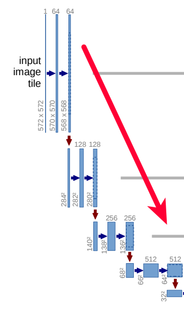
The downwards path in the U-Net architecture.
The downwards path is rather simple. In each chunk, we apply two 3x3 convolutions without padding, so 2 pixels are lost at the borders in each step. After each convolution, using the ReLU activation function (for more info on ReLU see training a simple neural network with plain numpy) is applied.
After 2 convolutions, a max-pooling operation with stride 2 is applied to halve the size of the image while keeping the same number of channels. Then with the next convolutions, the feature number is doubled.
So while going downwards, the image gets smaller and smaller while the feature channels get larger and larger.
A typical downwards step looks like this in Keras:
conv1 = Conv2D(64, 3, activation="relu", name="conv1_1")(inputs)
conv1 = Conv2D(64, 3, activation="relu", name="conv1_2")(conv1)
pool1 = MaxPooling2D(strides=2, name="max_pool1")(conv1)
Upwards path
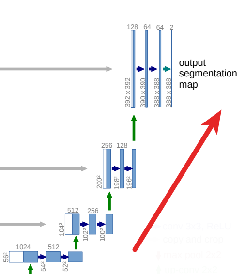
The upwards path in the U-Net architecture.
The upwards path is the opposite of the downwards path. While going up, the number of feature channels gets smaller while the size of the image increases again.
This is achieved by using so-called up-convolutions. This is the combination of an UpSampling2D layer in Keras which when used with size=2 doubles the size of the image and a regular 2x2 convolution which is used to halve the number of feature channels.
Another interesting property of the U-Net is that it combines layers from the downwards path with the upwards path by concatenation.
Cropping layers for concatenation
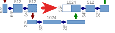
Concatenation in the U-Net architecture.
To be able to combine a downward layer with an upward layer, both the height and width have to match. However, due to the loss of border pixels with every convolutional layer, the height and width is larger in the downwards path than in the upwards path.
Thus, the downwards path needs to be cropped appropriately. I wrote a small function which calculates the proper crop values called determine_crop.
Basically, we take the difference in height and width between our target (which is the larger slice from the downwards path) and the goal (which is the smaller slice from the upwards path) and divide it equally, so the same amount of pixels is cut from the top, bottom, left and right.
def determine_crop(target, goal):
  height = (target.get_shape()[1] - goal.get_shape()[1]).value
  if height % 2 != 0:
    height_top, height_bottom = int(height/2), int(height/2) + 1
  else:
    height_top, height_bottom = int(height/2), int(height/2)

  width = (target.get_shape()[2] - goal.get_shape()[2]).value
  if width % 2 != 0:
    width_left, width_right = int(width/2), int(width/2) + 1
  else:
    width_left, width_right = int(width/2), int(width/2)

  return (height_top, height_bottom), (width_left, width_right)
The result of our determine_crop function can then be fed directly to a Cropping2D layer in Keras.
Example:
We want to combine a goal slice from the upwards path and a target slice from the downwards path.
Let’s say our goal slice has a size of 56x56 pixels in 512 channels.
Our target slice from the downwards path measures 64x64 pixels in 512 channels.
Therefore, determine_crop(target, goal) = ((4, 4), (4, 4)), so we cut 4 pixels from each side of target which transforms it from 64x64 to 56x56 pixels.
Then we can concatenate the goal slice with the cropped target slice to get a final concatenation size of 56x56 pixels in 1024 channels.
A typical upwards step looks like this in Keras:
up_sample1 = UpSampling2D(size=2, name="up_sample1")(conv5)
up_conv1 = Conv2D(512, 2, activation="relu", padding='same', name="up_conv1")(up_sample1)
height, width = determine_crop(conv4, up_conv1)
crop_conv4 = Cropping2D(cropping=(height, width), name="crop_conv4")(conv4)
concat1   = Concatenate(axis=3, name="concat1")([up_conv1, crop_conv4])
conv6 = Conv2D(512, 3, activation="relu", name="conv6_1")(concat1)
conv6 = Conv2D(512, 3, activation="relu", name="conv6_2")(conv6)
The full code for building U-Net in Keras
from keras.models import Model
from keras.layers import Conv2D, MaxPooling2D, Input, UpSampling2D, Cropping2D, Concatenate

inputs = Input((572, 572, 1), name="input") # starting with 572x572 pixels in a single color dimension

conv1 = Conv2D(64, 3, activation="relu", name="conv1_1")(inputs)
conv1 = Conv2D(64, 3, activation="relu", name="conv1_2")(conv1)
pool1 = MaxPooling2D(strides=2, name="max_pool1")(conv1)

conv2 = Conv2D(128, 3, activation="relu", name="conv2_1")(pool1)
conv2 = Conv2D(128, 3, activation="relu", name="conv2_2")(conv2)
pool2 = MaxPooling2D(strides=2, name="max_pool2")(conv2)

conv3 = Conv2D(256, 3, activation="relu", name="conv3_1")(pool2)
conv3 = Conv2D(256, 3, activation="relu", name="conv3_2")(conv3)
pool3 = MaxPooling2D(strides=2, name="max_pool3")(conv3)

conv4 = Conv2D(512, 3, activation="relu", name="conv4_1")(pool3)
conv4 = Conv2D(512, 3, activation="relu", name="conv4_2")(conv4)
pool4 = MaxPooling2D(strides=2, name="max_pool4")(conv4)

conv5 = Conv2D(1024, 3, activation="relu", name="conv5_1")(pool4)
conv5 = Conv2D(1024, 3, activation="relu", name="conv5_2")(conv5)

up_sample1 = UpSampling2D(size=2, name="up_sample1")(conv5)
up_conv1 = Conv2D(512, 2, activation="relu", padding='same', name="up_conv1")(up_sample1)

height, width = determine_crop(conv4, up_conv1)
crop_conv4 = Cropping2D(cropping=(height, width), name="crop_conv4")(conv4)
concat1   = Concatenate(axis=3, name="concat1")([up_conv1, crop_conv4])

conv6 = Conv2D(512, 3, activation="relu", name="conv6_1")(concat1)
conv6 = Conv2D(512, 3, activation="relu", name="conv6_2")(conv6)

up_sample2 = UpSampling2D(size=2, name="up_sample2")(conv6)
up_conv2 = Conv2D(256, 2, activation="relu", padding='same', name="up_conv2")(up_sample2)

height, width = determine_crop(conv3, up_conv2)
crop_conv3 = Cropping2D(cropping=(height, width), name="crop_conv3")(conv3)
concat2   = Concatenate(axis=3, name="concat2")([up_conv2, crop_conv3])

conv7 = Conv2D(256, 3, activation="relu", name="conv7_1")(concat2)
conv7 = Conv2D(256, 3, activation="relu", name="conv7_2")(conv7)

up_sample3 = UpSampling2D(size=2, name="up_sample3")(conv7)
up_conv3 = Conv2D(128, 2, activation="relu", padding='same', name="up_conv3")(up_sample3)

height, width = determine_crop(conv2, up_conv3)
crop_conv2 = Cropping2D(cropping=(height, width), name="crop_conv2")(conv2)
concat3   = Concatenate(axis=3, name="concat3")([up_conv3, crop_conv2])

conv8 = Conv2D(128, 3, activation="relu", name="conv8_1")(concat3)
conv8 = Conv2D(128, 3, activation="relu", name="conv8_2")(conv8)

up_sample4 = UpSampling2D(size=2, name="up_sample4")(conv8)
up_conv4 = Conv2D(64, 2, activation="relu", padding='same', name="up_conv4")(up_sample4)

height, width = determine_crop(conv1, up_conv4)
crop_conv1 = Cropping2D(cropping=(height, width), name="crop_conv1")(conv1)
concat4 = Concatenate(axis=3, name="concat4")([up_conv4, crop_conv1])

conv9 = Conv2D(64, 3, activation="relu", name="conv9_1")(concat4)
conv9 = Conv2D(64, 3, activation="relu", name="conv9_2")(conv9)

classes = Conv2D(2, 1, padding='same', name="classes")(conv9)

model = Model(input=inputs, output=classes)

model.summary()
Applications of U-Net
Now that you know how to build the U-Net in Keras, here are some example applications:
- Detect ships on satellite images - see Kaggle challenge
- Salt detection on spectral images
- Cancer detection on medical images
- Detection of organisms on biomedical images
machinelearning imagesegmentation medicalimages unet deeplearning
Machine Learning Deep Learning
1376 Words
February 27, 2019