Graphical Explanation of Neural Networks and Gradients with Python :: Päpper's Machine Learning Blog — This blog features state of the art applications in machine learning with a lot of PyTorch samples and deep learning code. You will learn about neural network optimization and potential insights for artificial intelligence for example in the medical domain.

How does an artificial neuron work?

Inspired by neurons of the human brain, an artificial neuron receives several input values.

These input values are multiplied with the weights of the neuron which reflects that some input values are activating the neuron (positive weights) while others inhibit the neuron (negative weights).

The product values are then summed and together create the activity a.

Finally, a non-linear function is applied on a to yield the final output of the neuron. In the human brain, this function is usually a threshold function, so the neuron fires when a is above the threshold and it doesn’t fire when a is below the threshold.

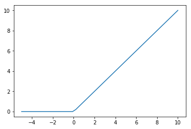
In artificial neurons, the ReLU (Rectified Linear Unit) activation function is rather popular, because it is simple and has good properties when it comes to the backpropagation of gradients. For ReLU negative values are set to 0 (rectified) and all other positive values are linearly passed through (linear unit).

Here it is as easy as it gets in one line of Python:

import matplotlib.pyplot as plt
import numpy as np
%matplotlib inline

def relu(x):
    return np.maximum(x, 0)
    
x = np.linspace(-5, 10)
plt.plot(x, relu(x))

png

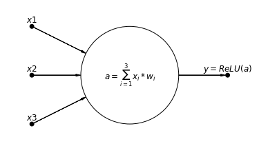
Plot of the neuron

To help grasp a neuron even more, let’s plot it. We let it take three input values $x_1$ - $x_3$ , calculate the activation as the sum of the multiplied inputs and weights and finally apply the ReLU activation function:

import daft
from matplotlib import rc
rc("font", family="serif", size=12)
rc("text", usetex=False)

pgm = daft.PGM((2.5, 1.35), origin=(-0.25, -0.15), grid_unit=5, node_unit=5)

pgm.add_node(daft.Node("input1", r"$x1$", 0, 1, fixed=True, scale=0.25))
pgm.add_node(daft.Node("input2", r"$x2$", 0, 0.5, fixed=True, scale=0.25))
pgm.add_node(daft.Node("input3", r"$x3$", 0, 0, fixed=True, scale=0.25))

pgm.add_node(daft.Node("neuron", r"$a=\sum_{i=1}^{3}{x_i * w_i}$", 1, 0.5))
pgm.add_node(daft.Node("output", r"$y=ReLU(a)$", 2, 0.5, fixed=True, scale=0.25))

pgm.add_edge("input1", "neuron")
pgm.add_edge("input2", "neuron")
pgm.add_edge("input3", "neuron")
pgm.add_edge("neuron", "output")

pgm.render()

png

Example calculation

After the graphical understanding, let’s make the calculations as explicit as possible with some example input values and weights:

x1 = 2; x2 = 3; x3 = 4
w1 = 1; w2 = -1; w3 = 5
a = x1 * w1 + x2 * w2 + x3 * w3
y = relu(a)
print(y)

19

Neural network in numpy

Now that we understand how a single neuron works, we can turn to a larger building block: the neural network.

An artificial neural network is basically just a mathematical function which takes input values and returns output values. However, the function can be arbitrarily complex - the network learns it using training data.

A neural network can consist of many different layers of neurons which led to the term “deep learning” for neural networks with many layers.

In the following example, we are creating a very simple neural network which consists of 2 layers. The first layer receives 1000 input values (input_dim) und calculates 100 output values (hidden_dim) on which we apply the ReLU activation function again.

The second layer receives the 100 output values of the first layer as input values and transforms them to a single final output value (output_dim).

The calculations for the neural network are done as for a single neuron, but since we now have several neurons, it is a matrix multiplication instead of a vector multiplication.

import numpy as np

batch_size = 128
input_dim = 1000
hidden_dim = 100
output_dim = 1

Random values

To show that such a neural network can learn an arbitrary mathematical function, we are creating random values - both for the inputs as well as for the outputs.

For the weights of our network which we want to learn over time, we are also starting at random and then adjust them step by step to get the expected result.

The perfect result would be to receive our random output_values when we pass in the random input_values.

We take a batch_size of 128 which means that we have 128 examples of 1000 inputs and 1 output.

input_values = np.random.randn(batch_size, input_dim)
output_values = np.random.randn(batch_size, output_dim)

weights1 = np.random.randn(input_dim, hidden_dim)
weights2 = np.random.randn(hidden_dim, output_dim)

First results

Let’s have a look how our randomly initiated network works right now:

Not very well, because our expected output_values were generated in the range -1 to 1, but our network computes values that differ by a few magnitudes. The error between our expected output and our actuval output is thus very high.

layer1_activations = input_values.dot(weights1) # inputs * weights1
layer1_relu = relu(layer1_activations) # apply ReLU
predictions = layer1_relu.dot(weights2) # intermediate output * weights2

print(predictions[:5] - output_values[:5]) # show difference of first 5 examples

[[ 48.29647842]
[-395.82459519]
[-198.78531708]
[-108.64914016]
[-279.01574778]]\

The good news is that we can use this high error, because we adjust the weights guided by the error. If the error is high, we make a bigger adjustment of the weights and if we error is low, we make a small adjustment.

The error can be represented as a function and we try to minify this function to get the error as small as possible. So we should adjust our values in the direction of the function to make the error smaller.

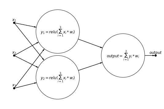
Plot of a neural network

Let’s make a small plot of a neural network which is much smaller than the one we defined in our example, but to make it clear how our example looks like approximately:

pgm = daft.PGM((3.55, 2.35), origin=(-0.25, -0.15), grid_unit=5, node_unit=5)

pgm.add_node(daft.Node("input1", r"$x_1$", 0, 1.75, fixed=True, scale=0.25))
pgm.add_node(daft.Node("input2", r"$x_2$", 0, 1, fixed=True, scale=0.25))
pgm.add_node(daft.Node("input3", r"$x_3$", 0, 0.25, fixed=True, scale=0.25))

pgm.add_node(daft.Node("neuron1", r"$y_2=relu(\sum_{i=1}^{3}{x_i * w_i})$", 1, 0.5))
pgm.add_node(daft.Node("neuron2", r"$y_1=relu(\sum_{i=1}^{3}{x_i * w_i})$", 1, 1.55))
pgm.add_node(daft.Node("neuron3", r"$output=\sum_{i=1}^{2}{y_i * w_i}$", 2.5, 1))
pgm.add_node(daft.Node("output", r"$output$", 3.25, 1, fixed=True, scale=0.25))

pgm.add_edge("input1", "neuron1")
pgm.add_edge("input2", "neuron1")
pgm.add_edge("input3", "neuron1")
pgm.add_edge("input1", "neuron2")
pgm.add_edge("input2", "neuron2")
pgm.add_edge("input3", "neuron2")
pgm.add_edge("neuron1", "neuron3")
pgm.add_edge("neuron2", "neuron3")
pgm.add_edge("neuron3", "output")

pgm.render()

png

Graphical meaning of minimizing the error function

So how exactly do we make the network learn?

We found out that we can calculate a loss function which is our error given our calculated results and our expected results.

The calculated results in turn depend on the weights in our neural network. If we change the weights, the results will change as well.

When using a method called gradient descent which is generally used to train such networks, we are calculating the gradients of the error by the weights and change the weights inversely proportional to their gradients.

That sounds complex, so let’s take a look why that makes sense!

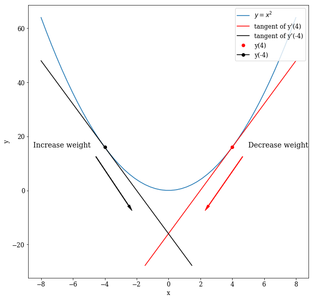
For illustration, we will turn to the quadratic function $y = x^2$ and assume that y is our error and x is a weight of the network. We can clearly see that the minimum of that function is at $x = 0$ which yields $y = 0$.

def y(x):
    return x * x

x = np.linspace(-8,8)

plt.figure(figsize=(10,10))
plt.plot(x, y(x), label='$y=x^2$')

png

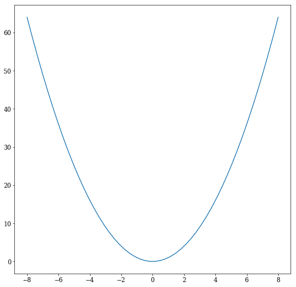
The derivative of the function (which is just the slope of the function at the corresponding points) is $y’ = 2*x$. It follows that: $x = 4 => y(4) = 16 => y’(4) = 8$ and $x = -4 => y(-4) = 16 => y’(-4) = -8$.

We will plot this scenario to make it graphically clear. It is graphically easy to see that for $x = -4$ the tangent is falling, so the derivative is negative ($y’(-4) = -8$) while for $x = 4$ the tangent is rising, so the derivative is positive.

When the derivative is negative, we are to the left of the minimum and thus need to increase our weight (x). An increase of x is achieved by subtracting the negative derivative. In contrast, when the derivative is positive, we are to the right of the minimum and thus need to move the weight (x) to the left which is also subtracting the derivative.

def y_derivative(x):
    return 2 * x
def tangent(x_0):
    return lambda x: y_derivative(x_0) * (x - x_0) + y(x_0)

plt.figure(figsize=(10,10))
plt.plot(x, y(x), label='$y=x^2$')
plt.plot(x[20:], tangent(4)(x)[20:], 'r', label='tangent of y\'(4)')
plt.plot(x[:-20], tangent(-4)(x)[:-20], color='black', label='tangent of y\'(-4)')
plt.plot([4], [y(4)], 'ro', label='y(4)')
plt.plot([-4], [y(-4)], marker='o', color='black', label='y(-4)')
plt.annotate('Decrease weight', xy=(2, -10), xytext=(5,y(4)), size=14,
            arrowprops=dict(color='red', width=1.0, shrink=0.1, headwidth=5))
plt.annotate('Increase weight', xy=(-2, -10), xytext=(-8.5, 16), size=14,
            arrowprops=dict(facecolor='black', width=1.0, shrink=0.1, headwidth=5))
plt.xlabel('x')
plt.ylabel('y')
plt.legend(loc='upper right')

png

The learning loop

We now have all necessary parts to train a neural network.

To do so, we are using a loop to run our training data (input_values) several times through the network. They are multiplied with the weights of the first layer (weights1) followed by the ReLU activation function. That result is then multiplied with the weights of the second layer (weights2) to get the final predictions of the network.

Our error is measured as the sum of squared differences between the predictions and the actual target values. Based on this error value, the different gradients for our weights are calculated (the mathematical details are not further explained here, but it basically works as explained above by using the chain rule in addition).

The gradients are used to change our weights a little bit (using a small learning_rate) in the right direction during each loop and thus reduce the error more and more.

num_loops = 500
learning_rate = 1e-6
for i in range(num_loops):
    activations = input_values.dot(weights1)
    relu_activations = relu(activations)
    predictions = relu_activations.dot(weights2)
    
    loss = np.sum(np.square(predictions - output_values))
    if ((i <= 100) & (i % 10 == 0) | (i % 100 == 0)):
        print(i, loss)
    
    # Gradients
    dloss_predictions = 2.0 * (predictions - output_values)
    dloss_weights2 = relu_activations.T.dot(dloss_predictions)
    dloss_relu_activations = dloss_predictions.dot(weights2.T)
    dloss_activations = dloss_relu_activations.copy()
    dloss_activations[activations < 0] = 0
    dloss_weights1 = input_values.T.dot(dloss_activations)
    
    # Adjust the weights
    weights1 -= learning_rate * dloss_weights1
    weights2 -= learning_rate * dloss_weights2

0: 9105954.33
10: 736508.54
20: 179914.40
30: 62107.40
40: 25320.33
50: 11819.75
60: 6066.79
70: 3340.08
80: 1938.26
90: 1171.71
100: 732.03
200: 65.96
300: 61.52
400: 61.51\

When comparing the final predictions of the network with our expectations we can now see that the errors are close to 0, so our network has learned good weights:

layer1_activations = input_values.dot(weights1)
layer1_relu = relu(layer1_activations)
predictions = layer1_relu.dot(weights2)

print(predictions[:5] - output_values[:5])

[[-1.33467775e-04]
[-6.36713506e-02]
[ 1.01669034e-10]
[-1.74870686e-06]
[-1.49639101e-09]]\