7 minutes
Interactive visualization of stable diffusion image embeddings
A great site to discover images generated by stable diffusion (or their custom model called aperture) is Lexica.art.
Lexica provides an API which can be used to query images matching some keyword / topic. The API returns image URLs, sizes and other things like the prompt used to generate the image and its seed.
The goal of this blog post is to visualize the similarity of images from different categories in an interactive plot which can be explored in the browser.
Lexica’s API
So let’s start off by getting images of a certain concept from Lexica:
import json
import requests
from pathlib import Path

def get_image_list_for(concept: str, n: int = 10):
    """ Get the first `n` results for `concept` from Lexica """
    url = f"https://lexica.art/api/v1/search?q={concept}"
    response = requests.get(url)
    if response.status_code == 200:
        return response.json()['images'][:n]
    else:
        raise Exception("Invalid response from Lexica")
The API is straigthforward - you just make a GET request for the concept you are interested in and you receive a list of matching images.
With this implementation, we can for example call get_image_list_for('dogs', n=5) to get Lexica’s info on 5 dogs.
A single entry of one of these dog entries would look like this:
{'id': '001b5397-...', 'gallery': 'https://...', 'src': 'https://...', 'srcSmall': 'https://...', 'prompt': 'a dog playing in the garden', 'width': 512, 'height': 512, 'seed': '3420052746', 'grid': False, 'model': 'stable-diffusion', 'guidance': 7, 'promptid': '394934d...', 'nsfw': False}
The gallery entry is Lexica’s URL to the gallery of this image where several other related images are shown, the src and srcSmall are the actual image URLs in two different qualities, seed, model, prompt and guidance are details about how the image was generated.
Download of images
Then let’s write some code to download the actual images from the src entries and also save them with the name of the concept plus some indexing number:
def save_image(url: str, path: Path):
    response = requests.get(url)

    if response.status_code == 200:
        with open(path, "wb") as f:
            f.write(response.content)

def download_concept(concept: str, n: int = 10):
    """ Gets `n` entries of `concept` and saves all the images as
    `concept`0.jpg - `concept`n-1.jpg as well as `concept`.json
    """
    data = get_image_list_for(concept, n)

    for idx, img in enumerate(data):
        path = Path.cwd() / f'{concept}{idx}.jpg'
        save_image(img['src'], path)

    path = Path.cwd() / f'{concept}.json'
    with open(path, "w") as f:
        json.dump(data, f)
So now when we call download_concept('dogs', n=5) the function will download the first 5 dog images which Lexica returns to us and store them as dogs0.jpg, dogs1.jpg etc. In addition, we also store the full API result in dogs.json.
Embedding the images with CLIP
To check how similar images are, we can embed them using the CLIP model which represents each image with 512 numbers. Then using those embeddings, we can cluster them and see which ones are actually similar to one another.
So let’s setup CLIP after installing some dependencies (pip install -U torch datasets transformers):
from transformers import CLIPProcessor, CLIPModel
import torch

device = "cuda"
model_id = "openai/clip-vit-base-patch32"

processor = CLIPProcessor.from_pretrained(model_id)
model = CLIPModel.from_pretrained(model_id).to(device)

def embed_images(img_list):
  with torch.no_grad():
    images = processor(
        text=None, images=img_list, return_tensors='pt')['pixel_values'].to(device)
    return model.get_image_features(images)
Now we have a method embed_images which takes a list of PIL Images and returns the embeddings of each image.
We can combine downloading images and embedding them:
from PIL import Image

def download_and_embed(concept: str, n: int = 10):
    download_concept(concept, n)
    imgs = [Image.open(f"{concept}{i}.jpg") for i in range(n)]
    embedded = embed_images(imgs)
    path = Path.cwd() / f'{concept}.pt'
    torch.save(embedded, path)
When we call download_and_embed('dogs', n=5) we will use the Lexica API to download 5 images of dogs, save them to disk, run them through the CLIP model and save their embeddings as dogs.pt.
Data Download
So we are almost there now, we just need to download a couple different categories to make it more interesting:
import os

n = 10
concepts = ['cat', 'dog', 'dinosaur', 'elephant', 'lion', 'mouse',
            'apple', 'banana', 'tomato', 'potato', 'pear', 'watermelon']
for concept in concepts:
  download_and_embed(concept, n)
After this, we have 10 images for each of our 12 categories with their embeddings stored locally. Great!
Now comes the fun part: visualization.
Visualization t-SNE
To visualize, we will take all of our embeddings and put them together into a single embedding data structure, so that we can then compute their similarities:
def get_single_embedding_tensor_of(concepts):
  tensor_list = []

  for filename in [Path.cwd() / f'{concept}.pt' for concept in concepts]:
      tensor = torch.load(filename)
      tensor_list.append(tensor)

  # Normalize by vector l2_norm to have them comparable
  embedded = torch.cat(tensor_list, dim=0)
  l2_norm = torch.norm(embedded, dim=1, keepdim=True)
  return embedded / l2_norm

all_emb = get_single_embedding_tensor_of(concepts)
All embeddings are stored in the variable all_emb which is of size (120, 512) - 120 images with 512 embedding dimensions.
Note that we normalized by the l2_norm to have their values be easily comparable.
Let’s check out the t-SNE plot of this data structure:
from sklearn.manifold import TSNE
import matplotlib.pyplot as plt
from matplotlib.patches import Patch
import numpy as np

tsne = TSNE(n_components=2)
tsne_embeddings = tsne.fit_transform(all_emb.cpu().numpy())

num_classes = len(concepts)
colors = plt.cm.rainbow(np.linspace(0, 1, num_classes))

class_labels = [i // n for i in range(all_emb.shape[0])]
color_list = [colors[label] for label in class_labels]

patches = [Patch(color=colors[i], label=cls) for i, cls in enumerate(concepts)]

fig = plt.figure(figsize=(10, 8))
plt.scatter(tsne_embeddings[:, 0], tsne_embeddings[:, 1], c=color_list)
plt.legend(handles=patches, loc='center left', bbox_to_anchor=(1, 0.80))
plt.show()
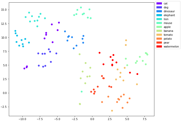
t-SNE plot of the embeddings with the classes as labels
Ok good, there is some overlap here and there for example between cats and dogs and for some of the edibles, but there are some clear clusters as well.
To have a comparison with t-SNE let’s also consider a UMAP plot after installing it with pip install umap-learn:
Visualization UMAP
import umap

umap_embeddings = umap.UMAP().fit_transform(all_emb.cpu().numpy())

fig = plt.figure(figsize=(10, 8))
plt.scatter(umap_embeddings[:, 0], umap_embeddings[:, 1], c=color_list)
plt.legend(handles=patches, loc='center left', bbox_to_anchor=(1, 0.85))
plt.show()
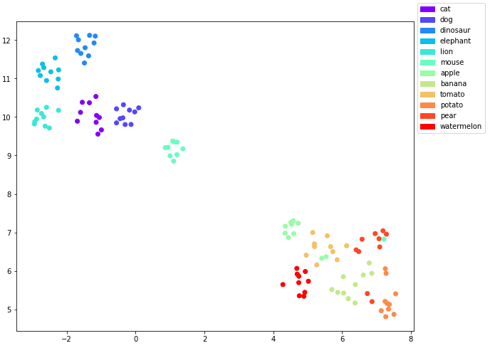
UMAP plot of the embeddings with the classes as labels
So that looks even a bit cleaner than the t-SNE plot. All the animal clusters are clearly separated in the upper left of the graph while the edibles are in the lower right.
For the edibles there is still some overlap between some of the points.
It would be interesting to figure out which images are overlapping here to get a better understanding about this. What we are missing to do at the moment is to figure out which image belongs to which data point. And it would really be nice to see the images corresponding to our data points directly in our visualization.
So let’s make it more interactive!
Interactive visualization with Bokeh
To do so, we will first base64 encode the images, so we can embed them in HTML:
import base64
from io import BytesIO

image_bytes = []
for concept in concepts:
  for i in range(n):
    image = Image.open(f"{concept}{i}.jpg").resize((256, 256))
    buffer = BytesIO()
    image.save(buffer, format='JPEG')
    image_byte = base64.b64encode(buffer.getvalue()).decode('utf-8')
    image_bytes.append(image_byte)
And then we use bokeh to make a cool interactive plot:
from bokeh.plotting import figure, show
from bokeh.models import ColumnDataSource, HoverTool
from bokeh.io import output_notebook

color_names = ['red', 'blue', 'green', 'yellow', 'purple', 'black',
               'grey', 'pink', 'orange', 'turquoise', 'cyan', 'brown']
color_lst = [color_names[label] for label in class_labels]

class_names = [concept for concept in concepts for _ in range(n)]

data = {'x': umap_embeddings[:, 0], 'y': umap_embeddings[:, 1],
        'color': color_lst, 'class': class_names, 'image': image_bytes}

fig = figure(tools='pan, wheel_zoom, box_zoom, reset')
fig.scatter(x='x', y='y', size=12, fill_color='color', line_color='black',
            source=ColumnDataSource(data=data), legend_field='class')

hover = HoverTool(
    tooltips='<img src="data:image/jpeg;base64,@image" width="256" height="256">')
fig.add_tools(hover)

output_notebook()
show(fig)
Try it out yourself!
When you hover over a data point, you will be able to see the stable diffusion generated image corresponding to it as retrieved from Lexica (you can also open it as its own page here):
Embeddings analysis
Now that we can identify how the images look like, we can have a closer look at the cluster outliers:
- A single mouse appears clustered together with the pears. It turns out that it’s a computer mouse and its shape resembles a pear a little bit:
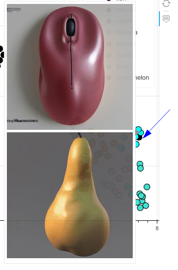
Mouse found inside the pear cluster
- Some apples get confused with tomatoes - if they are red and round, kind of makes sense:
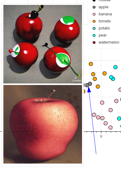
Some apples look like tomatoes
- Two pears dance out of line and get clustered closer to potatoes and bananes than their pee(a)rs, not really sure why (if you have an idea, please comment):
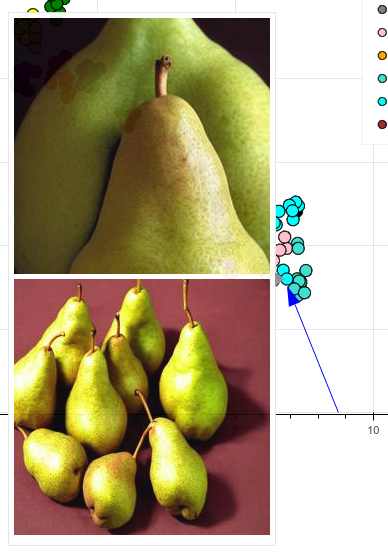
Pears dance out of line
Overall, I’m quite impressed that the semantic space is so well represented and concepts cluster quite tightly together.