5 minutes
Semantic segmentation with prototype-based consistency regularization
Semantic segmentation is a complex task for deep neural networks, especially when limited training data is available. Unlike image classification problems such as Imagenet, semantic segmentation requires a class prediction for every individual pixel rather than just an image-level class. This requires a high level of detail and can be difficult to achieve with limited labeled data.
Obtaining labeled data for semantic segmentation is challenging, as it requires precise pixel annotation, which is time-consuming for humans. In order to maximize learning from a limited set of annotated images while leveraging other non-labeled images, the paper “Semi-supervised semantic segmentation with prototype-based consistency regularization” by Hai-Ming Xu, Lingquio Liu, Quichen Bian, and Zhen Yang focuses on this problem.
Intuition of the approach
One of the biggest challenges with limited annotated data is overfitting, as the pixel-based information from labeled images is not easily generalizable. To address this issue, Xu et al. propose two segmentation heads: a standard linear prediction head and a prototype-based prediction head. A consistency loss is employed to encourage consistency between these two heads.
In semantic segmentation, the variation within the same class can be significant. For example, in the “person” class, there can be pixels for the head, hands, feet, etc. which all look quite different.
The prototype approach involves representing each class with multiple prototypes rather than learning to predict from features to a class in a matrix multiplication. This way, there can be a prototype for the head and another one for the hand in the “person” class.
When a linear classifier learns to correctly predict a class C from features (a, b, c) where a and b are features indicative of the class and c is irrelevant, then the linear classifier will learn to put a low weight on c.
In contrast, a prototype will have c as a relevant dimension as well and cannot undo that, so by ensuring consistency between both, the neural network can learn to rather set the feature c low in this case rather than the weight of c and by this it generates a better representation.
Method
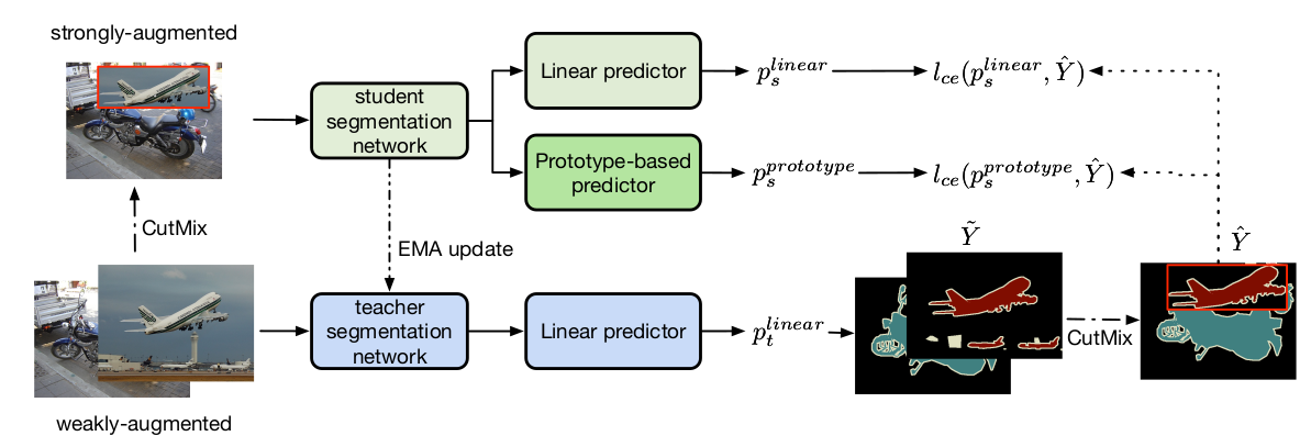
Figure 1 taken from the paper - illustration of the method, see explanation below in text.
Their semi-supervised approach works like this (Algorithm 1 + 2 in the paper):
- Prototypes are initialized:
- They first train in a regular supervised fashion with the available labels
- Then feature representations are extracted from the trained network by sampling a certain amount of pixels for each class
- K-means clustering is used on the sampled representations for each class to create K clusters.
- For each cluster, the features of it are averaged to obtain K prototypes per class.
- Train on a labeled and unlabeled set with a student and teacher network
- The student network uses two segmentation heads (linear and prototype head) and is trained using gradient descent
- The teacher network uses only the linear head and is an exponential moving average of the student (very slow moving)
- Each batch is sampled with 50% labeled and 50% unlabeled data
- For the labeled data, the student network is updated using standard gradient descent
- For unlabeled data:
- the teacher generated pseudo-labels using weak augmented versions of the images
- the student gets a strong augmented version using CutMix and is updated based on the teacher’s predictions (pseudo-labels)
- The prototypes are updated based on ground truth labels and pseudo-labels
- The update is done with a parameter alpha which controls how much of the old representation to keep (here alpha = 0.99)
- The currently learned feature representation is added to alpha times the old representation (1-alpha) times.
- The pseudo-labels are only used when their prediction confidence is larger than the parameter tau (see below)
To check for each pixel which class it belongs to in the prototype setting, cosine similarity is used. The prototype with the highest similarity to the pixel determines its class assigment.
In addition, a temperature parameter is used for the softmax based prototype similarity which is set to 0.1 to make the distribution sharper, i.e. closer to argmax.
The parameter tau controls which predictions of the teacher are actually used for training the student. Tau can be considered a confidence parameter, so if a prediction probability is larger than tau, it can be used for training the student. Phrased differently, each prediction of the teacher must be larger than tau, so the confidence is high that it will be a good target label for the student. In the paper, tau is set to 0.8.
The model they are using is a ResNet-101 backbone with a DeepLabv3+ decoder with a batch size of 16 (trained on 8 V100 GPUs).
Results
Results look convincing especially the less annotated data you have available where they beat supervised baselines by a large margin and also other semi-supervised methods.
Here is an example result for training on the PASCAL VOC 2012 data set with mean intersection over union (mIoU) as the relevant target metric on the validation data:
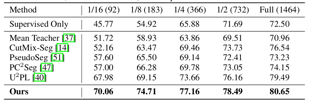
Table 1 taken from the paper - mIoU on PASCAL VOC 2012 val data.
Note that compared to the “supervised only” approach, they use several additional images without the labels to get this significant boost of performance.
In addition to numerical results, a t-sne plot of the data distribution is provided which compares the supervised only approach with the proposed approach without prototypes and with the full proposed approach. It can be seen that for some classes, the prototypes lead to a much compacter representation:
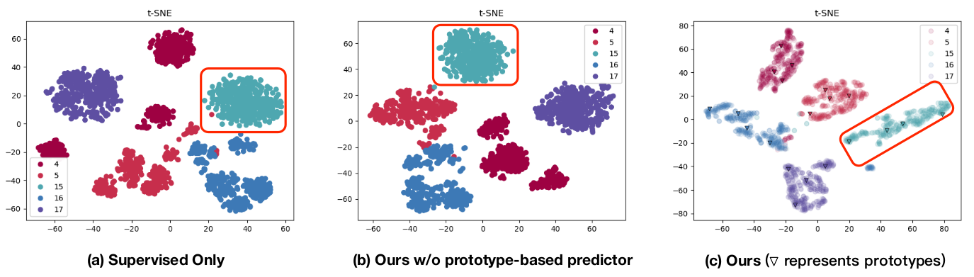
Figure 2 taken from the paper - compactness of person class (red outlined box) is better when using prototypes.
machinelearning deeplearning prototypes segmentation
Machine Learning Deep Learning Papers
929 Words
January 29, 2023