15 minutes
Everything you need to know about stable diffusion
The goal of this article is to get you up to speed on stable diffusion. You will learn the main use cases, how stable diffusion works, debugging options, how to use it to your advantage and how to extend it.
I) Main use cases of stable diffusion
There are a lot of options of how to use stable diffusion, but here are the four main use cases:
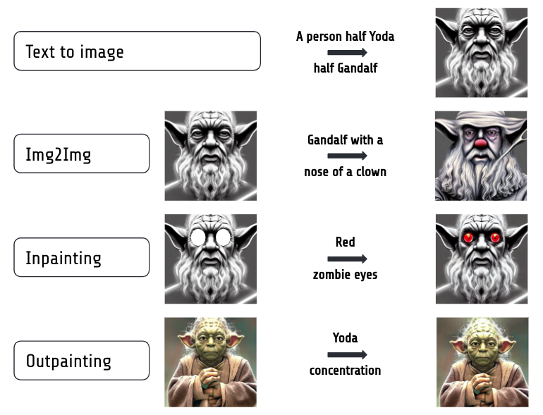
Overview of the four main uses cases for stable diffusion. See text for details.
- Text-to-Image: the classic application where you enter a text prompt and SD generates a corresponding image.
- Image-to-Image: tweak an existing image. You provide an image and a prompt and SD uses your image and tweaks it towards the prompt.
- Inpainting: tweak an existing image only at specific masked parts. You provide the image, a binary mask (with the areas to change) and a prompt. In the example below only the eyes are masked, so the rest of the image is not affected. Compare this with image-to-image where a lot of the image changes.
- Outpainting: add to an existing image at the border of it. You provide the image, the directon of where to extend it (e.g. 64 pixels to the top) and a prompt. For this one it’s usually best if you already generated your first image with stable diffusion and you have the prompt and seed you generated it with. It’s great to repair cut off heads etc.
II) Recap: how does stable diffusion work
In case you haven’t read my previous blog post, here is the tl/dr of how stable diffusion works:
Stable diffusion consists of three main ingredients:
- A text embedding model
- A denoising model which predicts the noise given an image
- A variational autoencoder (VAE) which is used to make it fast
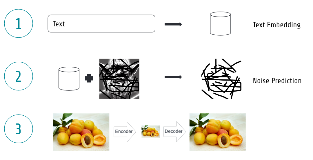
The three main ingredients of stable diffusion: 1) A text encoder to transform text to a vector 2) The denoising model predicting noise from images 3) A variational autoencoder to make it efficient.
1) Text embedding model
The text embedding model transforms a given text prompt into a machine digestible representation, a so-called embedding. And that is just a fancy name for a large dimensional vector which you know from high school. The cool thing about it is that it represents related text to related vectors, so the vector for “cute cat” will be very similar to the vector for “adorable cat”.
And how did we get such a cool model? It’s trained on millions of text-image pairs. Each text is passed through a text encoder model which spits out a text embedding and each image through the image embedding model which spits out an image embedding. Then during training you simply enforce to let the model learn that matching text-image pairs yield similar text and image embeddings while non-matching text-image pairs yield dissimilar text and image embeddings.
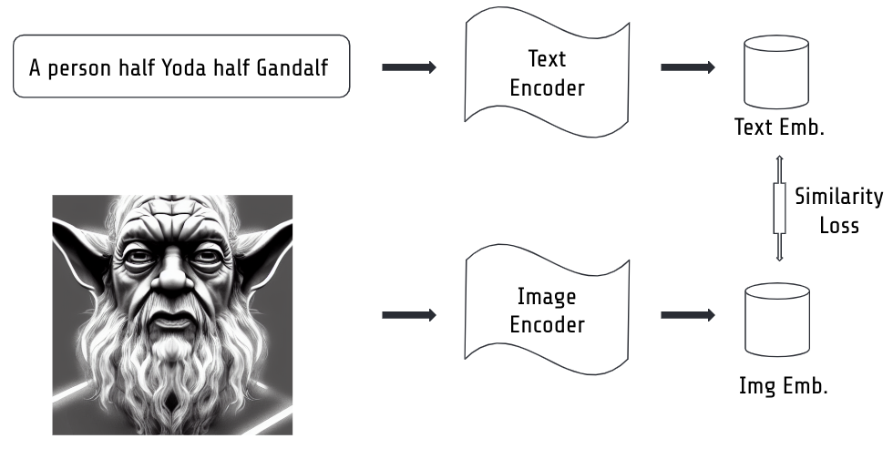
Illustration of how to train a text and image embedding model.
In the end you have both a great text embedder and a great image embedder. And for stable diffusion we need the text embedder.
2) The denoising model
The denoising model is at the core of the diffusion process. So you ask what is a diffusion process? During training we take an image and add noise to it in many steps. At each step, the image gets noisier. Then we train the denoising model (a U-net architecture) to predict the noise of a given image. As we have generated the noise ourselves, we know exactly what would be the perfect noise prediction, so we can then calculate a difference loss between the actual noise and the predicted noise and let the model learn from that until it’s quite capable to predict the noise well.
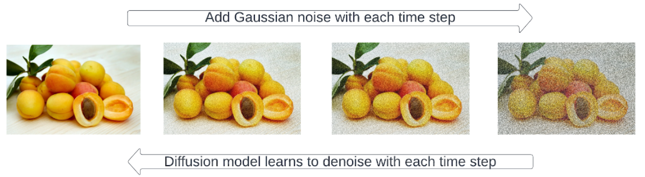
The illustrated diffusion process.
3) The variational autoencoder
The text embedding and the denoising model would be enough to do all this, but it would be SLOW. Stable diffusion generates images of 512x512 pixels in 3 colors, so that’s 786432 numbers per image. In the diffusion process we noise and denoise the image ~ 1000 times, so running this loop that often would be very expensive.
Luckily, the idea of Rombach et al. (https://arxiv.org/abs/2112.10752) was to move the whole image representation to a so-called latent space. The latent space is simply much smaller, so the whole denoising process becomes much faster.
How much faster you ask? Let’s see, the variational autoencoder consists of an encoder which transforms the 3x512x512 pixel image to a 4x64x64 pixel representation which is 16384 numbers, so only 2% of the original space.
Then once our denoising model has looped over the image several times in the latent space, we use the decoder to bring it back from 4x64x64 to 3x512x512 pixels.
Think of the VAE as a great compression and decompression algorithm which can encode images very efficiently in much less information to speed up the process massively.
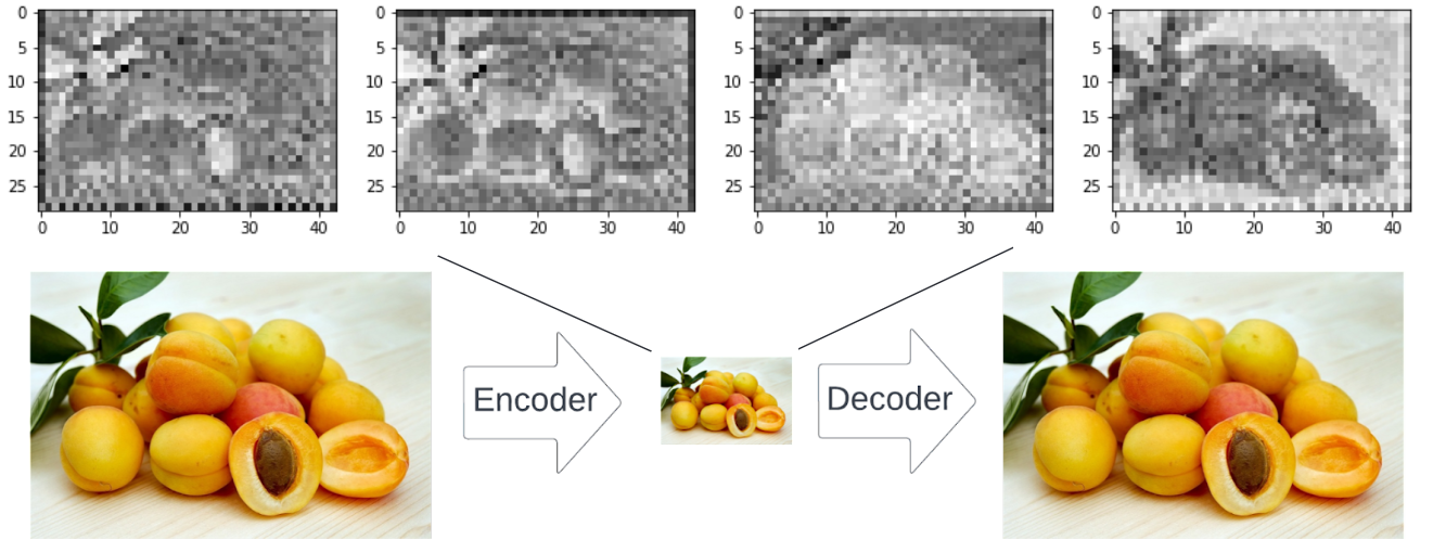
The VAE encodes images very efficiently. The small image of peaches is to understand the idea. In fact, it represents four channels in the latent space which are the black-and-white plots above.
The full inference description
With those three essential parts out of our way, we can take a look at how they are combined:
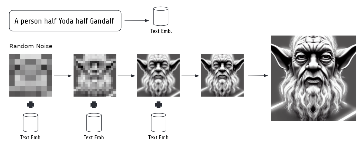
The full inference process of stable diffusion. Text is embedded. The embedding together with a random noisy image is fed to the denoising model several times in a loop. In the end the decoder of the VAE is used to go from the latent 4x64x64 pixel space to the 3x512x512 image space.
We feed the user entered text through the embedding model to receive a text embedding.
We generate random Gaussian pixel noise (which depends on the seed as we will learn later in this post) in our latent space of 4x64x64 pixels.
The random noisy image is passed to our denoising model together with the text embedding.
The denoising model predicts the noise it thinks is in the image (it uses the text embedding to guide it via cross-attention, see guidance scale below to boost it further).
We subtract the predicted noise from the noisy image and repeat this process several times (the number of repetitions is controlled by the steps parameter, read below).
In the end, we use the decoder part of our variational autoencoder to bring the 4x64x64 now denoised image back to our desired 3x512x512 pixel image space.
III) Debugging stable diffusion
The cool thing about attention values used in machine learning is that they are between 0 and 1, so if you have the attention values for the different words of your prompt, you can calculate their relative contributions and plot them in a histogram.
No need to build this yourself as the awesome diffusers-interpret library which builds on the fantastic diffusers library can do that for you!
So let’s take a look at the contributions of the different words in our prompt “Long-bearded wise old yoda with wizard powers”:
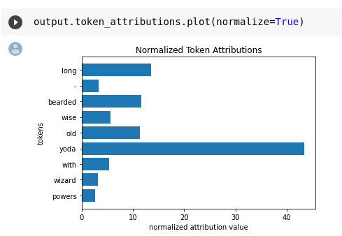
Attention attribution plot of the words in our prompt using diffusers-interpret.
You can see that a lot of attention went towards Yoda and quite a bit towards long, bearded and old. The reamining parts received little attention, so I don’t see many wizard features in this image (see gif below which constructs the image over time).
This can give you valuable clues as to where to tune your prompt to get a better representation of what you are aiming for.
And here is how stable diffusion generates the image for the prompt “Long-bearded wise old yoda with wizard powers” step by step:
SD inference steps visualized.
IV) How to tune stable diffusion
When you use stable diffusion from code or via an API, you usually have the ability to set certain parameters which define how your result turns out in the end. Let’s take a look at those with some explanations and visual examples:
The seed parameter of stable diffusion
The seed parameter makes up the random number generator state, so it will determine the initial noisy image which stable diffusion will try to denoise from. While you might think that generating initial noise would not have a big effect, think again. It is the initialization state which determines how the first steps turn out which then snowball into the later steps.
Essentially using a different seed will produce a very different image in the end. It will still represent the concept of the prompt, of course, but the style etc can be radically different:
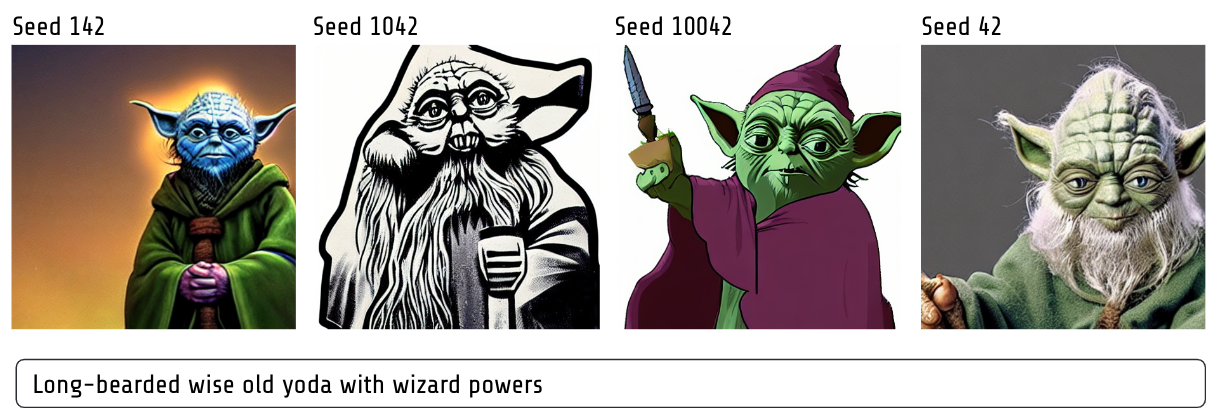
Different seeds lead to very different images.
The guidance scale / classifier free guidance
Classifier free guidance (CFG, https://arxiv.org/abs/2207.12598) is a technique to boost the impact of the text prompt.
In essence, stable diffusion is used once without the prompt and once with the prompt. In both cases, it tries to predict the noise from the image as good as possible. The “trick” here is to take the difference between the noise prediction including the prompt and the noise prediction without the prompt and then multiply this difference by the guidance scale.
Why does this make sense?
Well, the difference is the impact of the prompt on the noise prediction, so if we scale that difference we tell it to take that into account more, so to predict the noise matching our prompt more clearly.
The range of the guidance scale is 0-20 with a default value of 7.5. I think it usually makes sense to set it a bit higher to 8-14 to get better results. When you look at my example, you might even be tempted to set it higher than that, but if you set it too high, it easily generates some artifacts and you might not get as much diversity for different seeds.
Check in the image below how for the high CFG value of 20 when we let it run for 30 steps, the whole wave takes the shape of a cat. This might look cool, but it might not be what you want from the prompt.
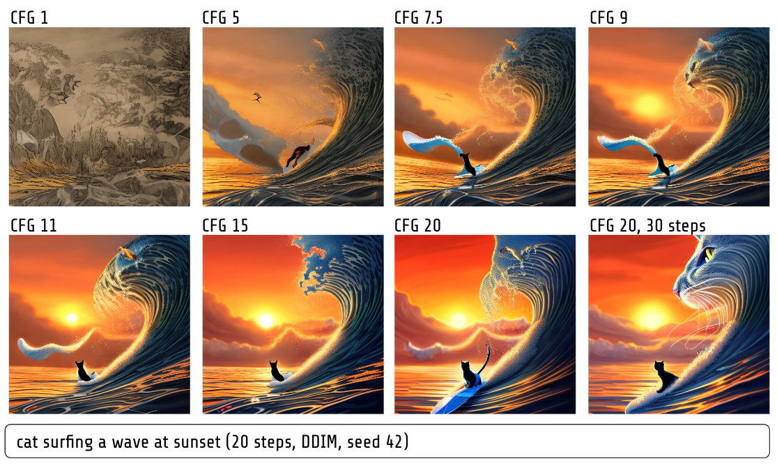
Impact of guidance scale on stable diffusion. All images are rendered with 20 steps except the last one to illustrate that with high guidance scales, sometimes the image gets morphed too much by your prompt.
Stable diffusion steps
The steps parameter is quite straightforward: it’s the amount of steps stable diffusion will repeat in a loop to denoise your image. Generally speaking, the more steps, the better the image quality. However, more steps = more compute = it takes longer and you pay more (GPU time). Also, there is a ceiling at some point where more steps will not make it better. Usually, 20-50 steps are enough for good quality, but sometimes you might want to go up to 100.
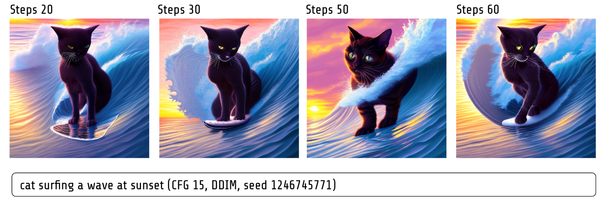
Impact of steps on stable diffusion. As you can see more steps are not always better.
Stable diffusion sampler
The details of samplers would be too much for this blog post, but the gist is that the samplers control the path through the latent space by setting the amount of noise at each step. I find that the difference between samplers is not so large, but there are some that are more efficient, i.e. they generate great images even for low step counts. I particularly like the DDIM sampler for this trait.
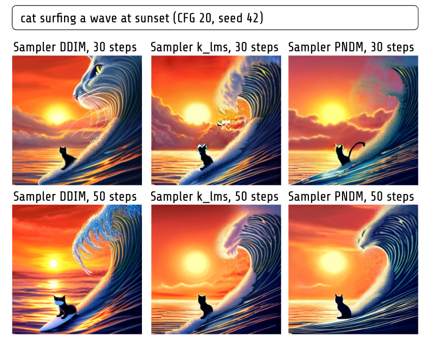
Effect of samplers at 30 vs 50 steps with high CFG. For k_lms and PNDM you can see blue artifacts for low step counts.
The prompt parameter
Of course, your prompt greatly influences the result. There are many tools out there which can help you with prompting.
Two I particularly like are Lexica for exploring images and their corresponding prompts and the promptomania prompt builder tool.
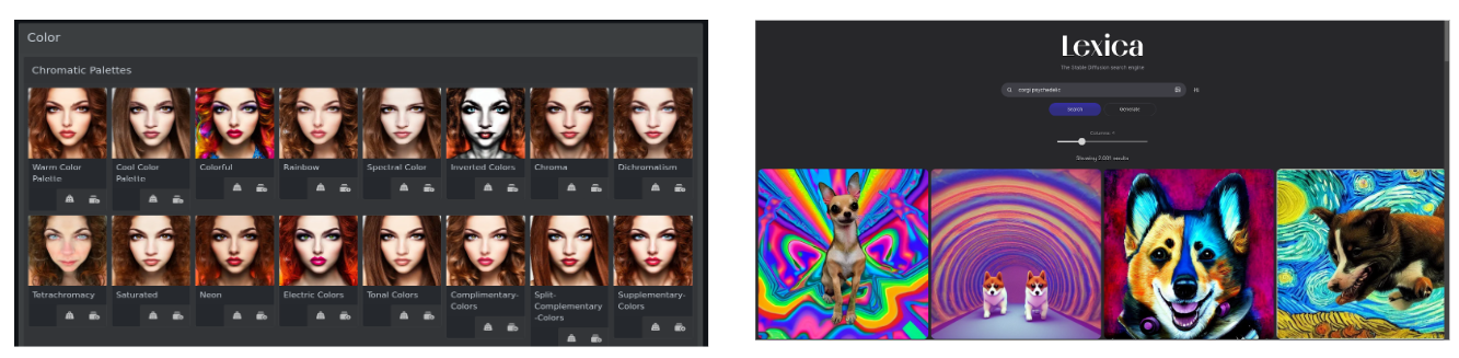
Images of two great tools to help with your prompts: Lexica and Promptomania prompt builder.
Recap important parameters
Here are the five most influential parameters of stable diffusion summarized in an image:
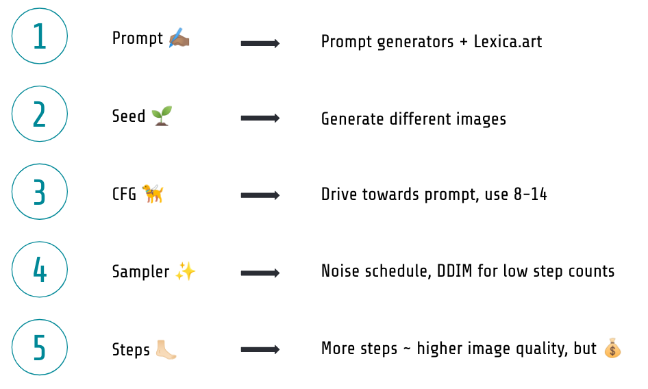
Most important stable diffusion parameters.
V) Extending stable diffusion
There are many more cool things you can do with stable diffusion and this section aims to explore a few of the options which are currently out there. Be sure, though, that there are a lot more (and a lot more to come!).
Mixing embeddings
As described above, our text embedding model generates a machine readable embedding for each word in our text prompt.
After it has been trained, it basically has learned a large matrix of word ID -> word embedding, so it looks up these embeddings.
One funny thing we can do is to take the embedding of multiple concepts / words and mix them with a linear interpolation.
Here is such an example where I replace the concept of dog with the mixed concept of squirrel and dog:
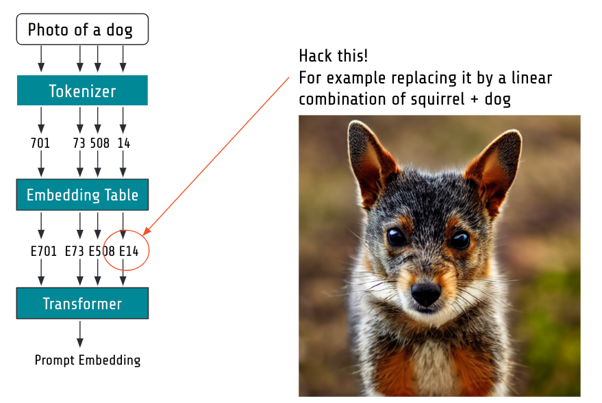
Mixing embeddings: here replace the embedding of dog with a linear combination of squirrel and dog.
If you want to play with this idea, start with this very helpful Fast.ai Jupyter notebook.
Textual inversion
If you want to go further than mixing embeddings, textual inversion has you covered.
It basically aims to learn a new text embedding covering your unique concept:
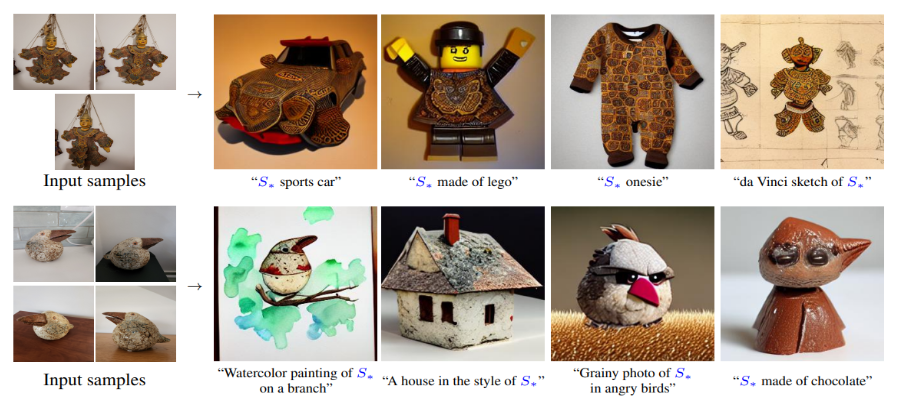
Textual inversion: examples, taken from the paper on https://arxiv.org/abs/2208.01618
To do so, you use a couple images of the concept you want to cover and textual inversion trains stable diffusion with backpropagation changing only your target embedding while the models are frozen.
That way during training, your unique embedding is learnt and associated with a special token denoted $S_*$ here. The training takes around 1 hour per new concept depending on your GPU.
You can then use $S_*$ in your prompts to generate new images with your special concept.
The cool thing about this is that you can share your token embedding with others, so you can mix and match with friends. Check out this concept library sharing textual inversion tokens.
This works, because the machine learning models are all kept untouched and only this token embedding is learnt:
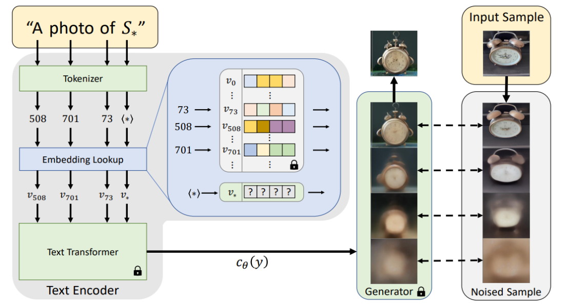
Textual inversion: illustration of method, taken from the paper on https://arxiv.org/abs/2208.01618
Imagic
Another super cool method is called Imagic. Imagic takes a picture and a prompt and transforms the picture to do what your prompt says while staying very consistent to the original picture.
Check out these examples to understand that intuitively:
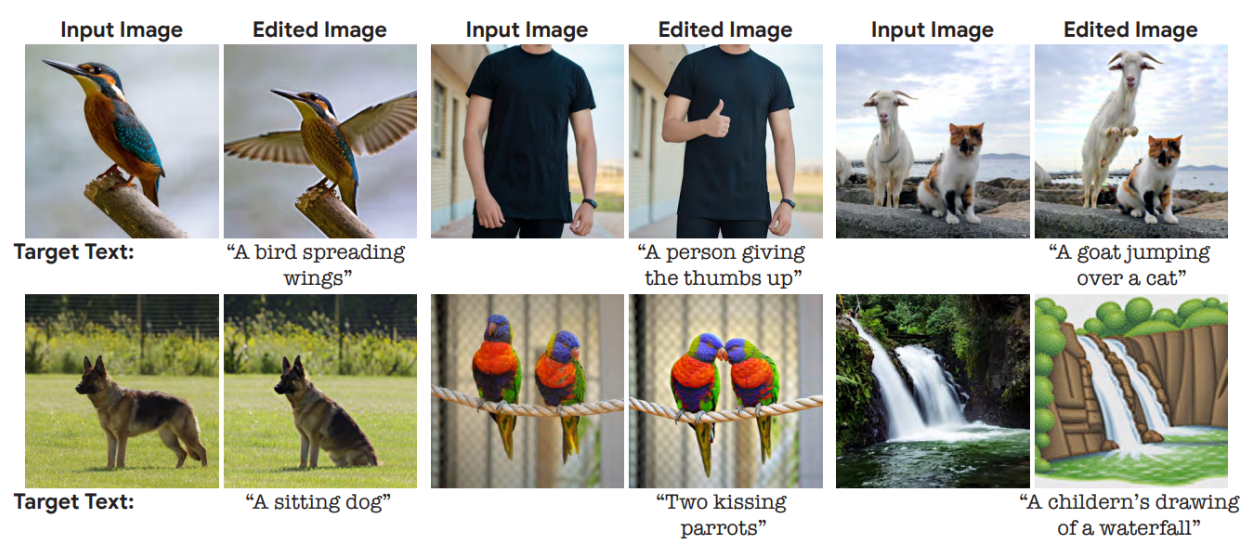
Imagic examples taken from https://arxiv.org/abs/2210.09276
The downside here is that you need to run a couple of steps involving training on the GPU, so it takes around 1 hour per image (depending on your GPU speed).
The procedure consists of these three steps:
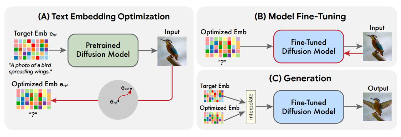
Imagic method taken from https://arxiv.org/abs/2210.09276
- You optimize your prompt text embedding to retrieve your original image - this is kind of like textual inversion with a single image.
- You fine-tune the denoising model to return the original image for your optimized text embedding.
- You make a linear interpolation of your original text embedding and your optimized text embedding and feed it through your fine-tuned model to get the result.
DreamBooth
The tool recently trending in social media with some services charging for it.
It’s similar to textual inversion in the sense that you provide images of a concept and then afterwards you can use a special prompt token to generate new images of your concept.
What is often used for DreamBooth are photos of yourself, so you can generate completely new pictures of yourself with different hairstyles or in different environments.
Let’s take a look at how it works first:
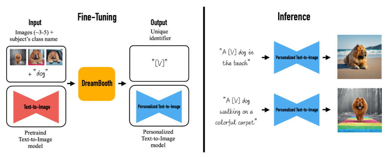
DreamBooth method taken from https://arxiv.org/abs/2208.12242
- You input images of your concept and a
class namefor your concept, e.g. ‘dog’ if you train on images of your dog or ‘woman’ / ‘man’ if you train on images of yourself. - The denoising model is fine-tuned using your provided images
- Other class specific images are used for regularization, so to not destroy the original creativity of stable diffusion as otherwise you’d risk overfitting
Of course, I couldn’t resist generating a couple of stable diffusion Marcs:
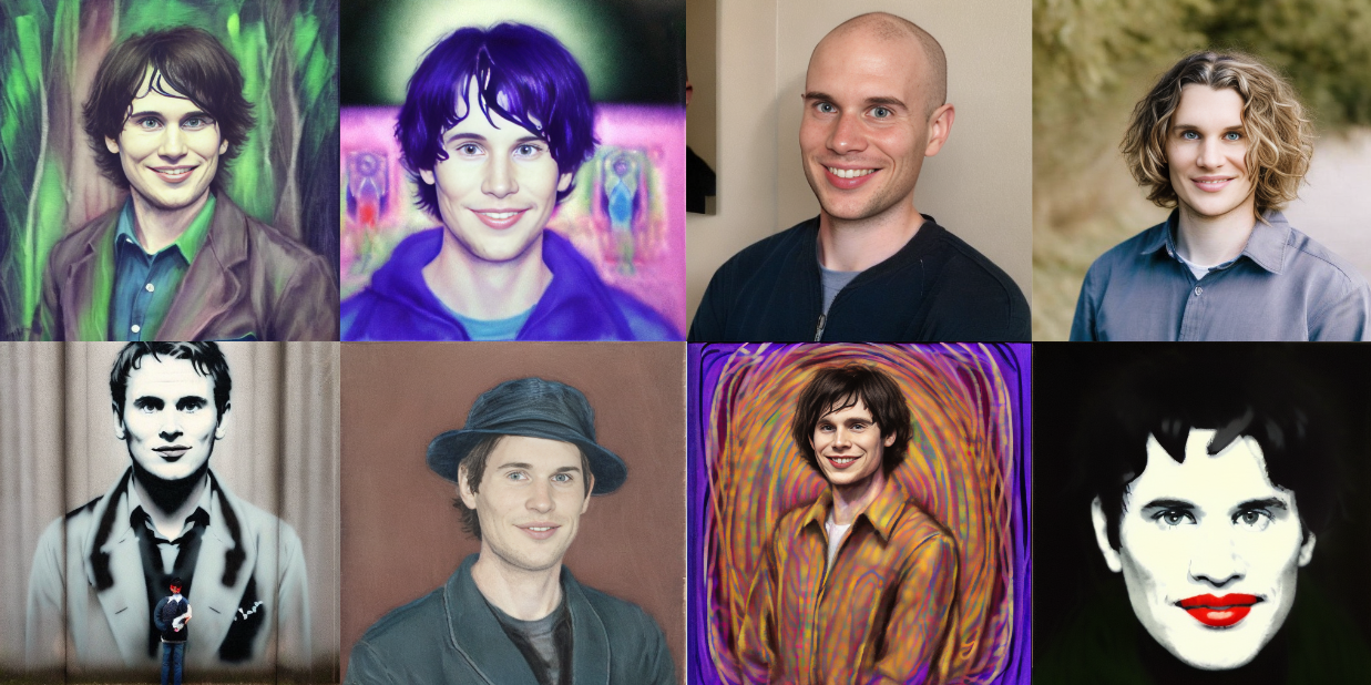
Stable diffusion fine-tuned on Marc via DreamBooth
Compared to textual inversion, the results tend to be a bit more advanced I’d say, but it has the downside that you fine-tune the whole model, so it’s not as easily shareable as the textual inversion concepts.
MagicMix
Another recent method is called MagicMix and the cool thing about it is that it needs no training, so it works out of the box just by changing the inference a little bit.
It is an extension of the basic image-to-image method which it improves upon.
It takes as input an image and a prompt and tunes the image towards the prompt.
You can check out my MagicMix implementation in this Jupyter notebook.
And here are some images generated with it:
Examples of MagicMix generated via https://github.com/mpaepper/stablediffusion_magicmix.
So let’s look at how it works:

MagixMix method taken from https://arxiv.org/abs/2210.16056
It consists of two phases:
a) The layout generation b) The fine-tuning or content generation
In a) it adds noise to the image you provide and keeps copies of the noised image at different time steps. In b) it uses the denoising model to denoise the noised image together with the embedded text prompt.
The trick is that in b) we always use a linear interpolation of the layout image from a) and the denoised version. That way, we can make sure that the rough layout of a) stays consistent, so we don’t deviate too far from the original image.
Conclusion
You should have a good overview of the current state of stable diffusion now as we covered the main use cases, how stable diffusion works, how you can debug it, what the important parameters are which you can control and some more advanced methods which build on top of it.
I hope this post will help you in understanding and working with stable diffusion. If you have any comments or questions, I would be happy to hear from you on twitter.com/mpaepper.
References
- Latent Diffusion Model paper by Robin Rombach, Andreas Blattmann, Dominik Lorenz, Patrick Esser, Björn Ommer: High-Resolution Image Synthesis with Latent Diffusion Models
- Classifier free guidance paper by Jonathan Ho, Tim Salimans: Classifier-Free Diffusion Guidance
- Textual Inversion paper by Rinon Gal, Yuval Alaluf, Yuval Atzmon, Or Patashnik, Amit H. Bermano, Gal Chechik, Daniel Cohen-Or: An Image is Worth One Word: Personalizing Text-to-Image Generation using Textual Inversion
- Imagic paper by Bahjat Kawar, Shiran Zada, Oran Lang, Omer Tov, Huiwen Chang, Tali Dekel, Inbar Mosseri, Michal Irani: Imagic: Text-Based Real Image Editing with Diffusion Models
- DreamBooth paper by Nataniel Ruiz, Yuanzhen Li, Varun Jampani, Yael Pritch, Michael Rubinstein, Kfir Aberman: DreamBooth: Fine Tuning Text-to-Image Diffusion Models for Subject-Driven Generation
- MagicMix paper by Jun Hao Liew, Hanshu Yan, Daquan Zhou, Jiashi Feng: MagicMix: Semantic Mixing with Diffusion Models
- Fast.ai grokking stable diffusion notebook by Jonathan Whitaker: Stable diffusion deep dive