4 minutes
Understanding the difference between weight decay and L2 regularization
Introduction
Machine learning models are powerful tools for solving complex problems, but they can easily become overly complex themselves, leading to overfitting. Regularization techniques help prevent overfitting by imposing constraints on the model’s parameters. One common regularization technique is L2 regularization, also known as weight decay. In this blog post, we’ll explore the big idea behind L2 regularization and weight decay, their equivalence in stochastic gradient descent (SGD), and why weight decay is preferred over L2 regularization in more advanced optimizers like Adam.
The Big Idea: Smaller Weights for Better Generalization
The big idea behind L2 regularization and weight decay is straightforward: networks with smaller weights tend to overfit less and generalize better. In other words, by reducing the magnitude of the model’s parameters, we can make it less prone to fitting the noise in the training data and improve its ability to make accurate predictions on unseen data.
Weight Decay: Reducing Weight Magnitude
Weight decay is a regularization technique that operates by subtracting a fraction of the previous weights when updating the weights during training, effectively making the weights smaller over time. Unlike L2 regularization which adds a penalty terms to the loss function (see below), weight decay directly influences the weight update step itself. This subtraction of a portion of the existing weights ensures that during each iteration of training, the model’s parameters are nudged towards smaller values. By gradually diminishing the magnitude of the weights, weight decay helps prevent overfitting and encourages the model to generalize better to unseen data. In mathematical terms, weight decay can be represented as a weight update step that subtracts a scaled version of the current weights, where the scaling factor is controlled by a small regularization parameter.
L2 Regularization: Adding a Penalty Term
L2 regularization, confusingly often also referred to as weight decay, involves adding a term to the loss function that penalizes the squared magnitude of the model’s weights. This term is usually represented as a fraction of the weight magnitude squared, multiplied by a small parameter. The goal is the same as for weight decay: encourage smaller weights to prevent overfitting. Due to the nature of calculating the gradients the squared weights term becomes just the regular weights term, so in the weight update step again a small fraction of the weights parameters are subtracted. That’s why alternatively for L2 regularization, the weight term is directly added to the gradients instead of its squared version to the loss.
Equivalence in Stochastic Gradient Descent (SGD)
In the context of SGD, weight decay and L2 regularization are equivalent. This equivalence arises from the fact that the gradient of the L2 regularization term leads to the same parameter update as the one applied in weight decay. Therefore, in vanilla SGD, using either weight decay or L2 regularization will achieve the same result in terms of weight updates. And this is exactly the reason why the two terms have been used synonymously.
Complex Optimizers and the AdamW Solution
However, things get more interesting when we consider more advanced optimization algorithms like Adam, which compute first and second moments of the gradients and use them to update weights. In these optimizers, the weight update depends on momentum parameters calculated after the gradients have been computed.
When L2 regularization is used with such optimizers, the regularization term gets transformed in the momentum calculation, making it no longer equivalent to simple weight decay. This transformation can lead to suboptimal results in practice.
The paper by Loshchilov and Hutter (Link to PDF) conducted several experiments showing that weight decay performs significantly better than L2 regularization when used with Adam and other adaptive optimizers. Consequently, researchers and practitioners now commonly use a modified version of Adam called AdamW, which incorporates weight decay directly into the optimizer.
Here is a nice illustration from the Loshchilov / Hutter paper which shows Adam and the changes that L2 regularization / decoupled weight decay apply:
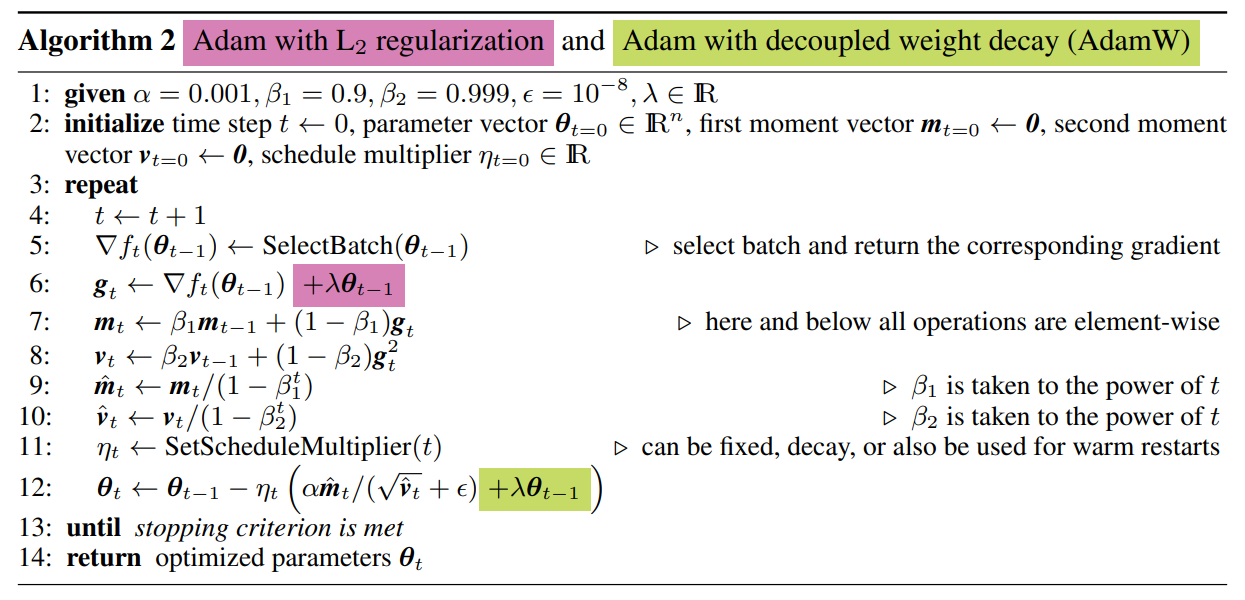
Figure from Loshchilov and Hutter comparing Adam for L2 regularization and weight decay.
As you can see, lines 7-10 are using the gradients in their calculation and then line 12 does the weight update. However, line 12 does the update not with the vanilla gradients, but with the computations from lines 7-10 and that’s exactly why L2 regularization is not the same as the decoupled weight decay update (which directly affects line 12 as visualized) for Adam.