10 minutes
How and why stable diffusion works for text to image generation
Stable diffusion is all the rage in the deep learning community at the moment. It’s trending on Twitter at #stablediffusion and gaining large amounts of attention all over the internet.
We’ll take a look into the reasons for all the attention to stable diffusion and more importantly see how it works under the hood by considering the well-written paper “High-resolution image synthesis with latent diffusion models” by Rombach et al which is the foundation of the system.
Reasons for stable diffusion gaining so much attention
In case you didn’t take a look at it, yet: stable diffusion is a text to image generation model where you can enter a text prompt like “A person half Yoda half Gandalf” and receive an image (512x512 pixels) as output like this:

Prompt: A person half Yoda half Gandalf, fantasy drawing trending on artstation
The results look like DALL-E 2 or even better which is awesome already on it’s own, but it gets even better: it’s very compute efficient and can run on a consumer GPU card needing only around 8-10GB of memory. It’s also more efficient than past models to train (alas still too expensive if you don’t have access to many GPUs).
On top of the computational efficiency, the results look splendid. In fact, as explained in the paper cited above, they reach several new highscores on image benchmarks such as image inpainting and class-conditional image synthesis.
And here comes the best part: this has been fully open-sourced. This includes the code, the model weights as well as the rights to use it for anyone with the goal to democratize creativity for anyone.
The stable part about it’s name stable diffusion is that the sponsor called Stability provided a lot of GPU compute to train this model to the current state (fine-tuned on 512x512px images) and then open sourced it.
If you want to try out some prompts yourself, you can do so on https://beta.dreamstudio.ai.
Looking under the hood: how does stable diffusion work?
I very much like hierarchical learning, so we’ll start with the high-level view and then go deeper on the individual parts.
High-level view
There are three parts to the system:
- A language model which transforms the text prompt you enter to a representation which can be fed to the diffusion model and used via cross-attention mechanisms. They use a “from the shelf” BERT tokenizer with a transformer for this part, so I won’t go deeper into it.
- The diffusion model which is basically a time conditional U-Net (for details on U-Net check here) which takes as input some Gaussian noise and the representation of your text prompt and denoises the Gaussian noise to get closer to your text representation. This is repeated several times that’s why it’s called time conditional.
- A decoder which takes the output of the diffusion model and upscales it to a full image. The diffusion model operates on 64x64px and the decoder brings this to 512x512px.
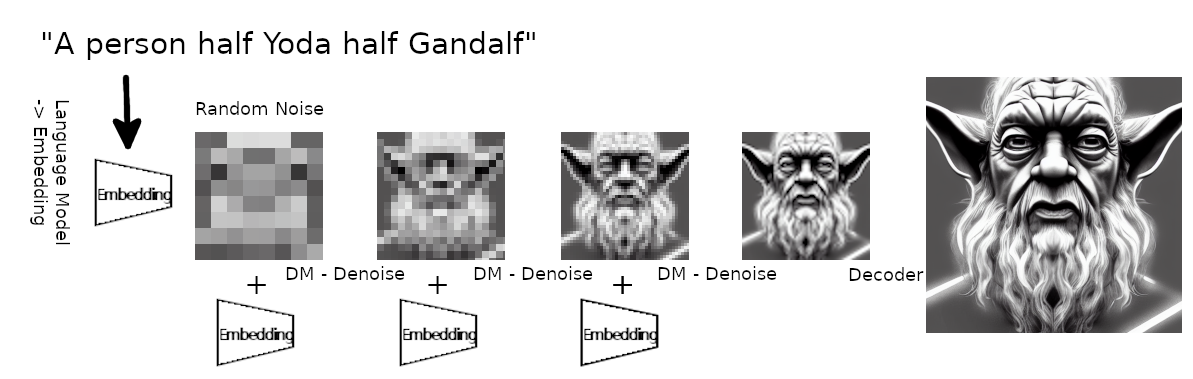
Illustration of the text to image generation (made by author). The language model creates an embedding of the text prompt. It’s fed into the diffusion model together with some random noise. The diffusion model denoises it towards the embedding. This is repeated several times. Then in the end the decoder scales the image up to a larger size.
High-level view of the diffusion model
The idea of diffusion models is that you take an image and add a little bit of Gaussian noise to it, so you obtain a slightly noisy image. Then you repeat that process, so to the slightly noisy image you again add a little bit of Gaussian noise to obtain an even noisier image. You repeat this several times (up to ~1000 times) to obtain a fully noisy image.
While doing so, you know for each step the original image (or slightly noisy image) and it’s noisier version.
Then you train a neural network which gets as input the noisier example and has the task to predict the denoised version of the image.
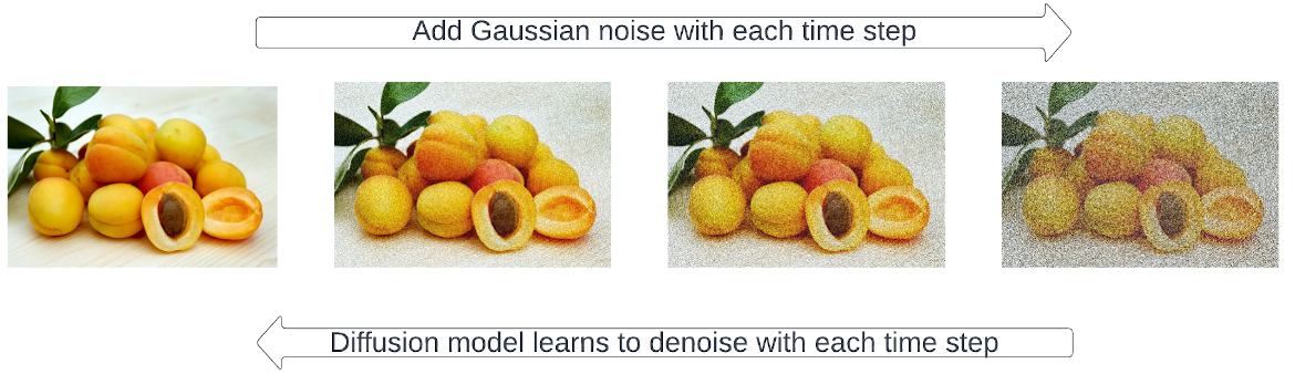
Illustration of the diffusion process (made by author): going from left to right you keep adding gaussian noise to your image. Then the model learns from right to left to denoise it.
In doing so for many different steps, the neural network learns to denoise very noisy images in a repeated manner to obtain the original image.
High-level training
During training, there also exists an encoder which is the counter-part to the decoder mentioned above.
Together, the encoder and decoder form an autoencoder.
The goal of the encoder is to transform an input image to a downsampled representation which has high semantic meaning but gets rid of high-frequency visual noise which is not very relevant to the image at hand.
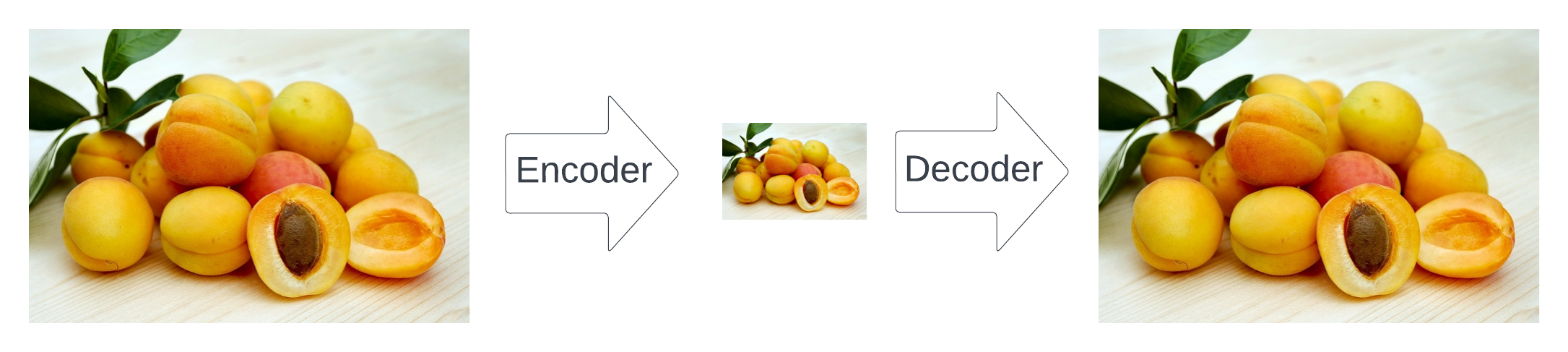
Illustration of the autoencoder (made by author): the encoder finds a much smaller representation of the image, but keeps the semantic meaning. The decoder regains the original version of the image from the efficient representation with as little loss as possible.
The trick here is that they decoupled the encoding from training the diffusion model. That way, the autoencoder can be trained to get the best image representation and then downstream several diffusion models can be trained on the so-called latent representation (that’s just the image represented in a semantically meaningful way, but with 64 times less pixels).
Doing so, the training of the diffusion model which is on pixel space needs to calculate 64 times less than before on the original image space. And this is totally relevant, because as we will see later, the training and inference of the diffusion model is the most expensive part.
So training progresses in two-phases:
- Training the autoencoder which handles compressing and decompressing the image representation
- Training the diffusion model on the latents generated by the encoder of the autoencoder (this is combined with the text representation / attention part)
Detailed view of the components
Training the autoencoder
The autoencoder is trained with two losses:
- A perceptual loss which is on the pixel space
- A patch-based adversarial loss which enforces local realism and avoids blurriness
It downsamples the image by a factor of f which has been tested in the paper with many different values and the trade-off of f=4 or f=8 was good.
In addition to the losses, regularization is applied to the autoencoder. There are two different forms which can be used here:
- A Kullback-Leibler penalty to align the learned latents towards the standard normal of the past latents to ensure that the variance in the latents is not too high
- A vector quantization layer within the decoder; this is like defining
Nprototypes
Sometimes they use the KL penalty, sometimes the vector quantization when training different diffusion models. To me it’s not fully clear when the one or the other is better. It seems that for the text to image synthesis model the KL penalty has been used.
Training of the diffusion model
Given the sequential number of steps to make an image noisy or in the inverse process to denoise it, this can be described as a Markov chain, because every time step only depends on the immediate successor and nothing else.
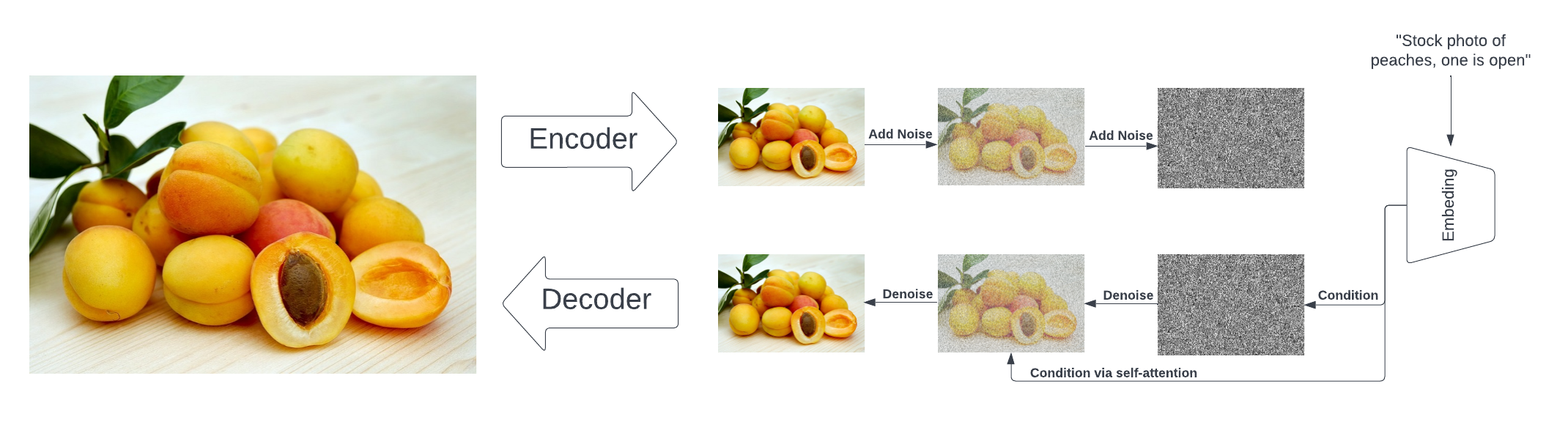
Illustration of the training process of the diffusion model (made by author). An image with existing caption is used for training. Noise gets added to the encoded image in successive timesteps. The text caption gets embedded by the language model. The diffusion model receives a noisy version of the image and the text embedding and needs to predict the previous time step of the image. Gradient descent is used on the pixel difference between the expected image and the prediction of the diffusion model.
To train it, you fortunately have the forward steps which can be generated efficiently, so you can for a given image know exactly how it looks noised at time step N and at time step N+1.
Then you pass the image at time step N+1 to the network and expect it to return the image at time step N. For the loss you consider the pixel wise difference between the network predictions and the image at time step N.
The more noise is on the image, the more the network spends on less relevant visual features, so typically more examples are sampled at earlier time steps than later time steps.
Wait, but why does this generate all this creative art?!
So the real question that you are asking yourselves, of course, is: where does the magic come from?
As I’ve described, it’s a complex system composed of three parts - the autoencoder, the language model for text embeddings and the latent diffusion model.
All of these parts are trained on a huge amount of images or image/text pairs, so the embeddings for the autoencoder and the language model are quite sophisticated and cover most of our human semantic space. When then combining concepts together via a new text prompt, the concepts get combined into an embedding that covers this. The latent diffusion model itself is trained to uncover an image out of noise, but guided by this embedding, so it drives the creative embedding concept towards an image representation. Then finally, the decoder helps to bring the latent representation to a more upscaled and human visible version (and it also is trained on millions of images!).
I think the magic is the overlap / composability of concepts which have been learned during training. For example some images were of half a man half a woman or something like that, so the concept of half / half was learned. Many other images contained parts of Star Wars / Yoda, so a concept of Yoda was learned. And then other images learned about Gandalf. When finally combining all of this into a prompt, the system tries to integrate all of this knowledge to the most likely image that could look like this. And thus images like the one in this article are created.
Summary
It was a great step forward to realize that to speed up a diffusion model, you should reduce the pixel space as that is used repeatedly (in the Markov chain approach) and thus gets expensive. In fact, it’s not only reducing the pixel space, but rather to learn a good representation / embedding by the autoencoder up front which still has all the semantics and also the visual representation of the semantics.
Doing so in a separated manner such that the autoencoder is trained separately makes it flexible to train several different diffusion models which are tuned towards special tasks.
Combining it with additional inputs in the cross-attention steps was critical to enable the mind blowing effect of having a fast and visually appealing text to image generation model.
However, instead of using text prompts, other input / embeddings can also be used. For example the authors show how to use a rough segmentation sketch map of classes which then gets transformed to beautiful images by the model and many more things such as removing a person from an image (think Photoshop magic wand super advanced tool):
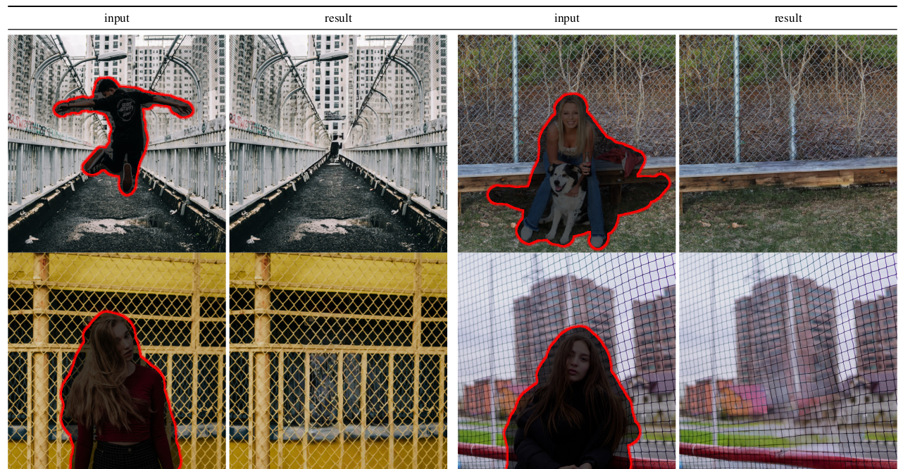
Taken from Figure 22 of the paper: latent diffusion model to remove objects from images.
Hopefully, this blog entry on stable diffusion gave you a good overview about the concepts used. If you are curious to go deeper, check out the latent diffusion model research paper on Arxiv.
Please let me know in the comments if this article was helpful for you or what you missed and how I might improve it in the future!
machinelearning deeplearning imagegeneration
Machine Learning Deep Learning Papers
1931 Words
August 27, 2022