6 minutes
Rethinking Depthwise Separable Convolutions in PyTorch
This is a follow-up to my previous post of Depthwise Separable Convolutions in PyTorch. This article is based on the nice CVPR paper titled “Rethinking Depthwise Separable Convolutions: How Intra-Kernel Correlations Lead to Improved MobileNets” by Haase and Amthor.
Previously I took a look at depthwise separable convolutions which are a drop-in replacement for standard convolutions, but focused on computational and parameter-based efficiency. Basically, you can gain similar results with a lot less parameters and FLOPs, so they are used in MobileNet style architectures.
In the current paper, the authors revisited the depthwise separable approach from a theoretical perspective and concluded that there might be even better ways which they then evaluated in several experiments.
General idea of the blueprint separable convolution
The idea (exactly like for depthwise separable convolutions) is that there are a lot of correlations between the different convolutional kernels we learn while training a neural network.
In the paper, several existing architectures are analyzed for such kernel correlations using a principal component analysis and the authors find that around 50% of each filter kernel’s variance can be explained by the first principal component.
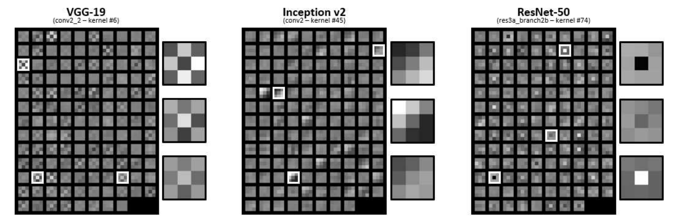
Figure 2 taken from the paper. Examples of correlations between convolutional kernels.
So given these intra-kernel correlations how can we make use of them?
The authors propose a blueprint approach which means that we learn the blueprint of a kernel and then scale it using also learned linear interpolation weights to derive all the correlated kernels. The linear interpolation weights are learned and can be both positive and negative.
That means that instead of learning CxO kernels, we only learn O kernels (called the blueprints) and then for each one learn C scaling factors.
That way you reduce the standard convolution’s CxKxKxO parameters to KxKxO parameters for the prototypes plus CxO weights to represent the C different kernels for each prototype.
Here is quite a nice visual explanation:
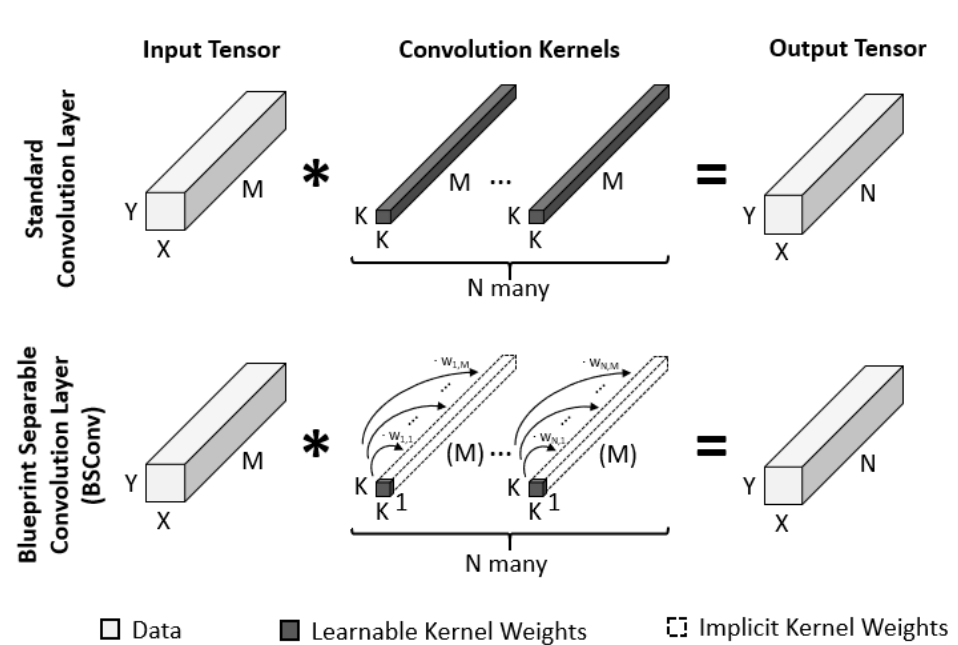
Figure 1 taken from the paper. For each output dimension (here N instead of O), we learn a single convolutional kernel. For each such blueprint, we learn weights to linearly scale it. Note that the weights can be both positive and negative.
Implementation of the blueprint approach
The authors derive an efficient implementation which consists of a pointwise convolution followed by a depthwise convolution. Interestingly, this is exactly the inverse of a depthwise separable convolution which combines a depthwise convolution followed by a pointwise convolution.
In the blueprint approach, the first pointwise convolution applies all the prototype weights, because it is not spatial, but combines the channels, so it learns one weight per channel (think of it as how much does this channel correspond to the blueprint) and then sums the channel weights.
In the depthwise convolution that follows, the spatial aspect is considered where the blueprints are applied over the previously determined linear combination of channel weights.
rethinking-depthwise-separable-convolution-illustration.png
Illustration of a blueprint separable convolution for a 3x3 kernel on a 3 channel input mapping to 6 output channels. For the blueprint separable convolution, first 1x1x3 (1x1 spatial x 3 input channels) points are mapped to a single point for each output yielding the same spatial structure as the input, but with 6 output channels. Then the depthwise convolution operations on 3x3x1 (3x3 spatial x 1 channel always) points which are mapped to 1 point each yielding 6 output points for the colored subset example.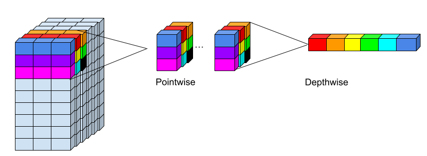
Implementation of the blueprint separable convolution in PyTorch
I’ll start with a standard convolution and then transform it to a blueprint separable convolution in PyTorch. To make sure that it’s functionally the same, we’ll assert that the output shape of the standard convolution is the same as that of the depthwise separable convolution. Of course, we also check the numbers of parameters which we are using.
from torch.nn import Conv2d

conv = Conv2d(in_channels=10, out_channels=32, kernel_size=3)
params = sum(p.numel() for p in conv.parameters() if p.requires_grad)

x = torch.rand(5, 10, 50, 50)
out = conv(x)

point_conv = Conv2d(in_channels=10, out_channels=32, kernel_size=1)
depth_conv = Conv2d(in_channels=32, out_channels=32, kernel_size=3, groups=32)

blueprint_conv = torch.nn.Sequential(point_conv, depth_conv)
p_blueprint = sum(p.numel() for p in blueprint_conv.parameters() if p.requires_grad)

out_blueprint = blueprint_conv(x)

print(f"The standard convolution uses {params} parameters.")
print(f"The blueprint separable convolution uses {p_blueprint} parameters.")

assert out.shape == out_blueprint.shape, "Size mismatch"
Generated output:
The standard convolution uses 2912 parameters.
The blueprint separable convolution uses 640 parameters.
As you can see, it’s easy and straightforward to implement and very similar to the depthwise separable convolution (just the inversion of pointwise and depthwise convolution; compare with the previous blog post).
Computational complexity
Given that the same operations are applied in inverse order as for the depthwise separable convolution, the number of learnable parameters and FLOPs are quite similar. The depthwise separable convolution is more expensive when the number of channels are higher in the previous layer than in the next layer while the blueprint separable convolution is more expensive when the number of channels are lower in the previous layer than in the next layer.
In architectures like MobileNet, the authors found a similar number of parameters for both operations which I think is due to mostly having the same number of channels in the previous and next layer.
In most architecures, the number of channels tend to rise with the depth of the network, so I’d consider the blueprint separable convolution to be a bit more expensive.
Results
The authors compare several models trained with and without their method.
Of course, when comparing their method with default CNNs, the number of parameters and FLOPs is much less, so I will focus on the comparison to existing networks which use the already optimized depthwise-separable convolutions.
Their results are quite impressive given that they achieve higher scores in all of their experiments across different tasks.
They argue that in contrast to the depthwise separable convolution which applies the depthwise convolution first, their method has access to all the channels in the beginning and this might be beneficial for visual tasks.
That said, as I mentioned before, the blueprint separable convolution is often slightly more expensive (at least FLOP wise), so it might be that there is some bias here which I have not experimentally verified at this point.
Summary
I reviewed blueprint separable convolutions which take a theoretical look at the depthwise separable convolutions and conclude that it might be worthwile to flip the point- and depthwise convolutions to go pointwise first before executing the depthwise convolution. This is theoretically validated by looking at intra-kernel correlations and then experimentally verified that it can actually also lead to better results.
They also argue that the depthwise separable convolution acts as a cross-kernel blueprint, so it assumes that there are necessary correlations between channels as well. Their method only uses intra-kernel correlations which is a bit weaker assumption, but also computationally slightly more expensive.
Their results are very good, so it’s definitely something to consider when trying out mobile optimized or smaller networks in general.
Something I didn’t cover here: other mobile architectures like EfficientNet use linear bottleneck blocks instead of depthwise separable convolutions. The authors also propose a blueprint option which is very related to linear bottleneck blocks and also show experimentally that it can have some gains.
I’d recommend reading the paper as it’s well thought out and well written.
machinelearning deeplearning convolution pytorch
Machine Learning Deep Learning Papers
1215 Words
July 19, 2022