8 minutes
Hyperparameter tuning on numerai data with fastai and weights & biases
Today we will try to tackle the Numerai tournament using the fastai deep learning library. However, as the results likely depend on many different hyperparameters, let’s take advantage of the weights and biases library and their sweeps API. Sweeps are hyperparameter runs which test out different combinations of your model’s hyperparameters.
What is Numerai?
Numerai is a hedge fund which trades stocks in a market neutral fashion. That means that they try to make money without having a lot of risk for their customers. Basically, whenever they buy or call a stock, they sell or short another one to counter-balance the risk.
The fun thing about Numerai is that they take advantage of an ensemble of data science predictions. To do so, they provide you with anonymized features (1050 currently) and a target column. It is a regression problem, so the target is between 0 and 1. You have a training, a validation and a test set. For the training and validation set, the targets are available. For the test set, you only have the features and need to predict the targets.
You then upload your predictions to Numerai (not your model!) and can bet money on the quality of your predictions (in terms of the cryptocurrency Numeraire). If your model turns out to be good, you’ll earn some more money back, but if your predictions were not good, some of your money will be burned / lost. Here, we are not interested in bidding money, but you can also upload your predictions and just see how you do over time.
Setting up fastai and wandb
First, we need to install our dependencies and import the basics from fastai and wandb:
!pip install wandb -q
!pip install fastai==2.5.3 -q
!pip install numerapi -q

import wandb
from fastai.tabular.all import *
Next, we download the data from Numerai, namely the training and the validation set. I download them in the _int8 format here to save some memory.
from numerapi import NumerAPI

napi = NumerAPI()
current_round = napi.get_current_round(tournament=8)  # primary tournament
napi.download_dataset(
  "numerai_training_data_int8.parquet", "numerai_training_data.parquet")
napi.download_dataset(
  "numerai_validation_data_int8.parquet", "numerai_validation_data.parquet")
Data preparation for fastai
Then let’s prepare the data for fastai. In fastai we usually have a single data frame for training and validation data, so I’ll merge them together and pass the indexes of the validation data for the data split:
import pandas as pd

train_df = pd.read_parquet(f'numerai_training_data.parquet')
val_df = pd.read_parquet(f'numerai_validation_data.parquet')

train_df = train_df.append(val_df).reset_index()
del val_df
val_idx = list(train_df[train_df['data_type'] == 'validation'].index)

feature_cols = [c for c in train_df if c.startswith("feature_")]
Metrics for numerai
In Numerai we are interested in having a high correlation of our predictions with the target. In particular, we are looking at eras which are points in time (we don’t know about the details) and the goal is to have a model which is robust over eras, because they are trading with money, so it’s better to be consistent over time rather than having a few eras with good performance and then incurring losses in other eras.
Thus, two important metrics which are generally used are the mean correlation of the eras and the sharpe ratio which is basically the mean divided by the standard deviation and should indicate how attractive your investment is (it’s more attractive when it has a good mean, but low standard deviation).
These helper functions can be defined like this:
from scipy.stats import spearmanr

def corr(df: pd.DataFrame) -> np.float32:
  corrs = df.groupby("era").apply(
    lambda d: spearmanr(d['target'], d['prediction'])[0])
  return corrs.mean()

def sharpe(df: pd.DataFrame) -> np.float32:
  corrs = df.groupby("era").apply(
    lambda d: spearmanr(d['target'], d['prediction'])[0])
  return corrs.mean() / corrs.std()
Defining the job to run for a weights and biases sweep
Now here comes the interesting part. we need to define a full training run which should also include the metric we want to optimize for.
As we want to see good results on the non-training data, we will of course use some validation metric to optimize for. One possibility would be to use the validation loss, but in this case, I’d rather go for one of the metrics we are actually interested in, so I chose the val_sharpe metric.
Note that I explicitly calculate this after each run and log it to wandb, using wandb.log({'val_sharpe': val_sharpe}).
So what exactly happens here?
We define a method called train() which can be called with a config object to define the hyperparameters which we want to have this run for. This will be called by wandb in the sweeps later on to test out many different hyperparams.
Inside the train() method, we initialize a wandb run using wandb.init() and make sure that wandb has the chance to override the config by using config = wandb.config.
Before and after each run we use the garbage collection and clean the cuda cache just to make sure that no unexpected memory leaks happen between runs.
We then use the set_seed(42, True) method from fastai to make the run reproducible. After all, otherwise, the randomization could have a larger effect than our hyperparameters between the runs. This is sth. you should also test and make sure that runs with the same hyperparameters in fact produce the same results.
Then, we initialize our data loaders, a tabular learner and fit using the one cycle method which fastai popularized. All the relevant hyperparameters are set using config.x, so for example config.epochs for the number of epochs to run for.
Finally, after the run is finished, we evaluate on our validation data and determine our correlation and sharpe values which we log to wandb.
import gc
from fastai.callback.wandb import *
def train(config=None):
with wandb.init(config=config):
config = wandb.config
gc.collect()
torch.cuda.empty_cache()
try:
set_seed(42, True)
dls = TabularDataLoaders.from_df(
train_df,
bs=config.batch_size,
cont_names=feature_cols,
y_names='target',
valid_idx=val_idx)
learn = tabular_learner(
dls,
wd=config.wd,
loss_func=MSELossFlat(),
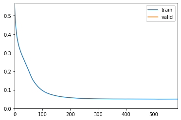
cbs=[ShowGraphCallback(), SaveModelCallback(), WandbCallback()])
learn.fit_one_cycle(config.epochs, lr_max=config.learning_rate)
prediction, target = learn.get_preds()
era = dls.valid_ds.items['era']
eval_df = pd.DataFrame({
'prediction': prediction.numpy().squeeze(),
'target': target.numpy().squeeze(),
'era': era}).reset_index()
val_sharpe = sharpe(eval_df)
val_corr = corr(eval_df)
wandb.log({'val_sharpe': val_sharpe})
wandb.log({'val_corr': val_corr})
print((f'Mean correlation: {val_corr}. Sharpe: {val_sharpe}.'))
except Exception as e:
print(e)
del learn
gc.collect()
torch.cuda.empty_cache()
Configuring wandb sweeps
The last step is now to tell wandb what to optimize for and which hyperparameters to try out.
In this case, I am using the bayes method which will try to figure out the optimal hyperparameters in a bayesian way (details are handled by wandb).
We define our val_sharpe as the metric with the goal to maximize it.
For the parameters we can either specify a concrete list of values like I did for the number of epochs or a range using min and max like for weight decay (wd).
For the sake of quickly running an example here, I am not using optimal values, but rather a small amount of epochs etc.
import wandb

sweep_config = {
  "method": "bayes",
  "metric": {
    "name": "val_sharpe",
    "goal": "maximize"
  },
  "parameters": {
    "epochs": {
      "values": [1, 2]
    },
    "wd": {
        "min": 0.01,
        "max": 0.1
    },
    "learning_rate": {
      "min": 0.001,
      "max": 0.01
    },
    "batch_size": {
      "values": [2056, 4112]
    }
  }
}

sweep_id = wandb.sweep(sweep_config, project='numerai-sweeps-blog')
Create sweep with ID: q7zn7a0s
Sweep URL: https://wandb.ai/mpaepper/numerai-sweeps-blog/sweeps/q7zn7a0s
Starting the weights and biases hyperparameter optimization
With this sweep_id we can now start agents to execute our runs - you could even do this from multiple machines to parallelize this.
We pass our train function to the agent and the count of experiments to run. I chose 10 here for the count, so we can get an idea. Normally, you would probably run at least 100 or more experiments. You can omit the count, so the agent runs indefinitely until you stop it.
wandb.agent(sweep_id, function=train, count=10)
The output will look something like this:
Sweep page: https://wandb.ai/mpaepper/numerai-sweeps-blog/sweeps/q7zn7a0s
| epoch | train_loss | valid_loss | time |
|---|---|---|---|
| 0 | 0.049930 | 0.050241 | 01:08 |
Better model found at epoch 0 with valid_loss value: 0.05024105682969093.
Validation correlation is: 0.012763993933631422. Validation sharpe is: 0.4141087498927619.
Waiting for W&B process to finish, PID 860… (success).
…and then continues for many runs.
Evalutating the results in weights and biases
Let’s take a look at some of the plots that we can get out of weights and biases to get insights about our problem. Again, here I ran with not the most sensible set of hyperparameters and only 10 runs, but we can probably already learn something.
The first nice thing we can get out of our runs is a feature importance weight table:
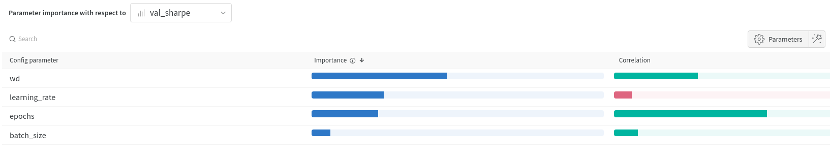
Feature importance weight table from wandb
We can see here that it seems to be beneficial for our val_sharpe metric to run more than a single epoch, to have some weight decay and also to use a larger batch size.
They are all positively correlated (green) with our target metric.
In contrast, the learning_rate is negatively correlated, so a smaller learning rate was better in our experiment.
Another great tool is the parallel coordinates panel in which you can define all the aspects you are interested in and you get a plot which shows all the different runs and where they end up finally. This is interactive on the wandb website, but here I’ve exported it as a png:
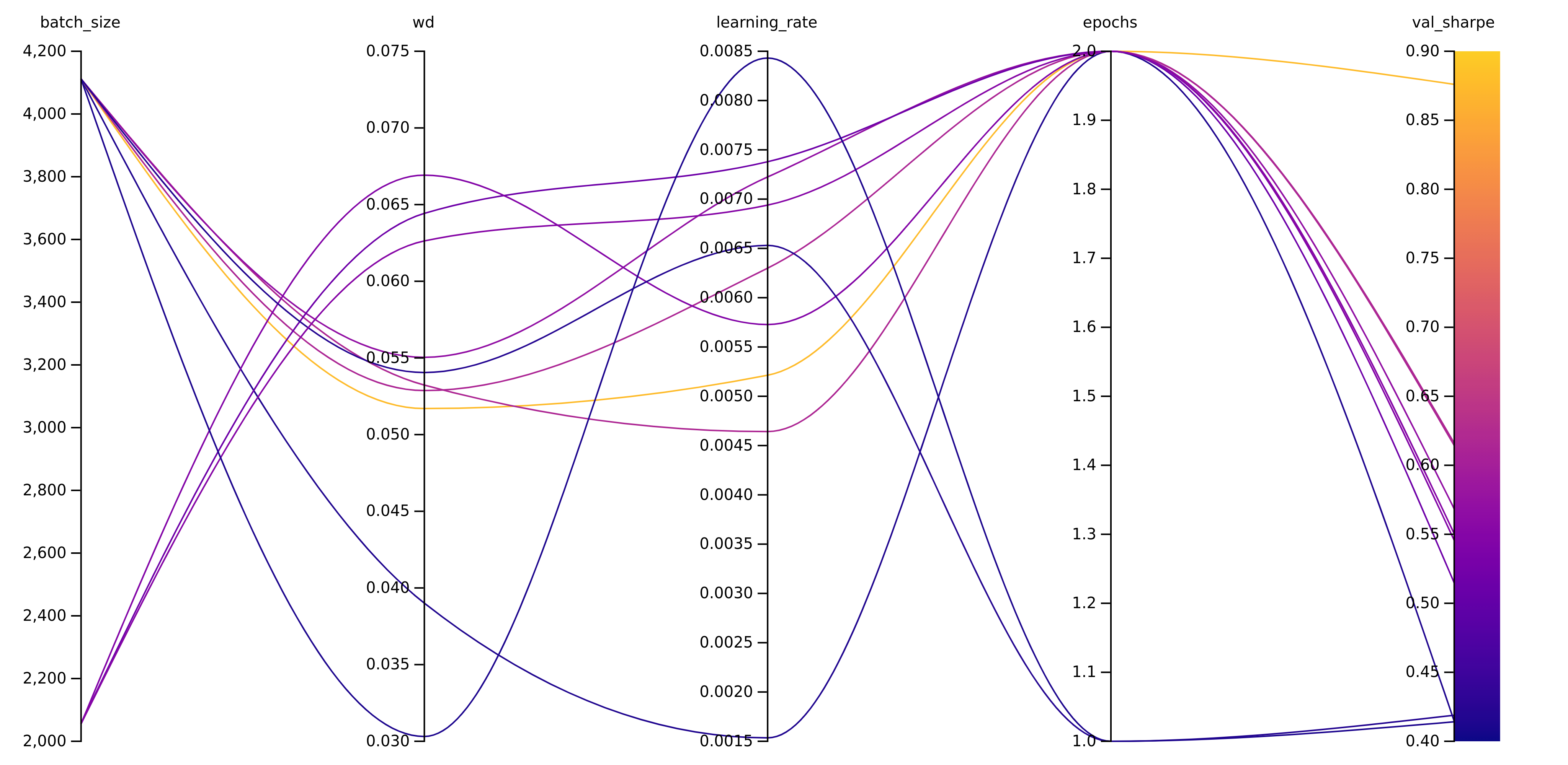
Parallel coordinates plot from wandb
We can see here that the run which finished with the highest val_sharpe value (yellow line) took advantage of a larger batch size and 2 epochs instead of 1 epoch while being somewhere in the middle of the weight decay and learning_rate scheme.
Summary wandb with fastai
To sum up: we could quickly start an experiment and easily tune the hyperparameters without a lot of work. Fastai enables us to quickly build a model with sensible defaults and the wandb hyperparameter sweeps are a very nice tool to collect the metrics of your different runs and generate some insights from different hyperparameters. What I like most about it: you can code it and then let it run over night. Then the next morning, you have all the results available and nice visualization tools at your hand.
python pytorch machinelearning deeplearning hyperparameters fastai wandb
Machine Learning Deep Learning
1630 Words
November 27, 2021