4 minutes
P-Diff Learning Classifier with noisy labels based on probability difference distributions
Label noise in digital Pathology
In the field of digital pathology and other health related deep learning applications, label noise is an important challenge to consider during training.
It’s inherent to the medical fields as the problems are extremely challenging even for trained experts, so there is high intra- as well as inter-observer variability.
This blog post dives into the idea of the paper P-DIFF: Learning Classifier with Noisy Labels based on Probability Difference Distributions which is authored by researchers of Microsoft in China. The idea is to use the probability outputs of your network during training to estimate the amount of noise and the particular noisy labels to exclude them and only train on non-noisy data.
P-DIFF values
If your model makes a wrong prediction during training, then it’s either because it hasn’t learned about a class properly, yet, or because the label of the class is wrong. With P-DIFF, we are trying to figure out this difference and use it to our advantage.
To do so, we consider the difference between the probability output of the target class and subtract the probability output of the next highest class probability. This is what’s called a probability difference or short P-DIFF.
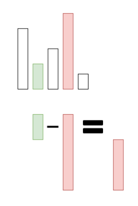
Let’s look at two examples to make this difference clearer!
We get a negative p-diff value if the probability of our target class (highlighted in green here out of our 5 class probabilities) is lower than the next highest probability of the distribution (red):
Example of a negative p-diff
In contrast, we get a positive p-diff value if the probability of our target class (green) is higher than the next highest probability (red):
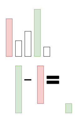
Example of a positive p-diff
Doing so, we get deltas in the range [-1, 1] where -1 happens when we predict 0 probability for the target class while being 100% sure it’s a wrong class. This indicates a likely candidate of a wrong label, because the network has learned sth. which it’s quite sure about, but the label totally disagrees. In contrast, a p-diff value of 1 indicates that the network assigned all the probability to the correct target class, so it perfectly learned to predict that example.
Here is a visualization of the p-diff value range:
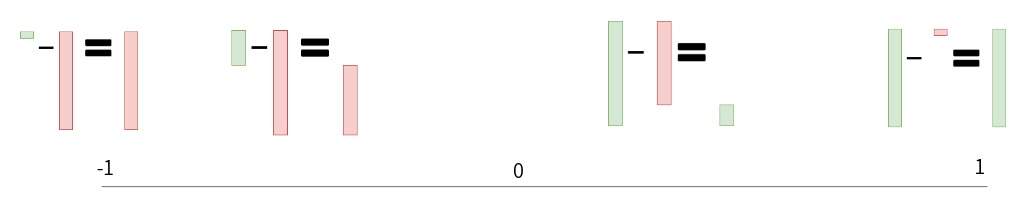
Visualization of p-diff range of values
So now we know how to compute these p-diff values, but how do we use them?
We plot them as a distribution and determine a cut-off threshold. Everything below that threshold is possibly noisy, so we only train on the data which is larger than the threshold.
At the start of the training, we have no idea about how to set the threshold, so we set it to -1 which means we are training on all the data. Then, for a number of warm-up epochs, we are slowly increasing the threshold up to 0 which would indicate that the network thinks another class is as likely as the target class.
We can even use the distribution to estimate the noise of the data by looking at the probability density which lies below the 0 threshold. This is used later in training when a value called zeta reaches a pre-defined threshold. zeta determines how strongly the distribution is divided into the tails of being very right about correct data and very wrong about potential noisy data.
And this is how the distribution changes over time during training:
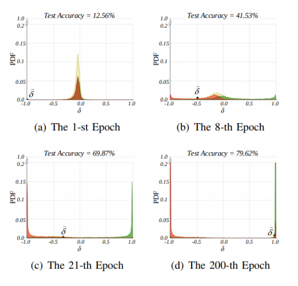
Figure 2 taken from the paper. The overall p-diff distribution is plotted in yellow over the duration of the training. It’s split into green (valid labels) and red (noisy labels), so we can see how they provide to the overall distribution. The threshold for deciding for noisy labels is plotted as delta here and as you can see it increases over time.
The adjustment for training is that in your loss function you introduce a weight. You set the weight to 0 for each example below your delta threshold and to 1 for each example above your delta threshold, so you essentially filter out the data which is deemed noisy.
Conclusion
P-DIFF is an easy to implement method which has low overhead in training time. This separates it from many other expensive label noise methods. That said, it has a somewhat heuristic character as you filter out data points which you don’t train on and you focus on others of the batch instead. This can lead to strange effects in case your problem is quite hard and inherently noisy as well.
What I really like about the approach is that you don’t need any additional data or special setup to implement it and you can nicely visualize the p-diff distribution and see whether it makes sense for your problem setup. Furthermore, it helps you to get an estimate of the noise rate of your labels which is a cool side effect.
In the paper, the authors show that it’s quite effective when introducing label noise to well-known problems like CIFAR-100 or Clothing1M.
References
Wei Hu, QiHao Zhao, Yangyu Huang, Fan Zhang: P-DIFF: Learning Classifier with Noisy Labels based on Probability Difference Distributions
python machinelearning deeplearning pytorch paper labelnoise
Machine Learning Deep Learning Deep Learning Papers
845 Words
October 17, 2021